This assignment will help you to appreciate the power of modern spreadsheet programs.  We will be using Microsoft Excel to parse data files, create plots of data, perform calculations, and visualize relationships defined by physically-based equations.  As you proceed with the following exercises, take some time to explore some of the features of the spreadsheet and try to imagine how you might use these features in your own scientific investigations.

Exercise 1-- Understanding the stresses surrounding magma chambers.

    The orientation of the maximum principle compressive stresses surrounding a magma chamber vary as a function of 1) the magnitudes of the remote principle stresses, and 2) the internal fluid pressure of the magma chamber.  We can idealize a magma chamber as a pressurized inclusion in an elastic plate and use mathematical solutions to this type of problem to see how the stresses vary around the magma chamber.
    The spreadsheet SPTRAJ.XLS is programmed to calculate the direction of the maximum compressive stress based on the remote principle stresses and the pressure of the magma chamber.  Open up this spreadsheet and try varying the magnitudes of the remote principle stresses and the magma chamber pressure to see what effect it has on the direction of the maximum principle stresses surrounding the magma chamber.  Take some time and use the spreadsheet to systematically explore how each of the parameters (sigmaxx, sigmayy, and p) effect the orientation of the maximum stresses around the magma chamber.  When you have gained some intuition about how these three factors effect the stress orientations, write a few paragraphs about the interaction of these three variables in creating the stress field that you see.
 

Exercise 2- Plotting first motions with Microsoft Excel.

    First motions of the earth's surface during an earthquake can give us clues as to the orientation of a fault surface as well as the type of displacement along the fault.  In this exercise, you will use Microsoft Excel to plot the first motion data from an earthquake near the San Andreas Fault, CA.  In the following data set, the first column is the Northing, the second column is the Easting and the third column is the first motion (D = dilation, C = compression).  You are to plot the data in Microsoft Excel and based on the knowlege of first motion data you gained in lab and your geologic knowlege of faulting, determine the type of fault that these motions indicate.

Data:

Northing        Easting        First Motion
0                         3                      D
-4                      10                      D
-2                      10                      C
-3                       2                       D
1                        0                       D
2                        0                       C
6                        5                       C
6                      20                       C

Write a paragraph describing what you think may be going on.  I understand that there is limited data here, but it should be enough to do a short first motion analysis.
 

Exercise 3-  Plotting the uplift surrounding a fault.

    On the Tejon public folder (PSF zone), you will find a file called GLG490--FaultExercise.xls.  Copy this file onto your computer.  This file contains data about the distribution of uplift surrounding a finite length, vertically dipping right-latteral strike-slip fault.  There are several relevant columns:  x1,x2,x3,u1,u2,u3.  The x1-x2 plane is the surface of the earth at x3=0 in this coordinate system.  x1 is easting, x2 is northing, and x3 is depth.  You will first need to parse the data file so that you can plot in Microsoft Excel. After you have done this, plot the uplift (u3) as a function of position in two dimensions (this will have to be done with a contour plot).  Save this contour plot as an Excel worksheet and submit it with the rest of the assignment.
 

Exercise 4-  Computing and plotting stream profiles in Microsoft Excel.

    Often, it is useful to plot the profile of a stream in order to understand the long-term development of the stream and what processes may be acting within the channel.  This can be applied to any topographic profile. The public disk on Tejon contains a data file called GLG490--Stream.xls.  Copy this file to your computer.  The file contains three columns:  Easting, Northing, and Elevation.  First, make a map view plot of the points.  Notice that they do not fall in a straight line.  When plotting a stream profile, we want to plot the elevation as a function of the down channel distance, L.  This distance is the distance between two points:
 

 

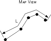
 L can be computed by using the Pythagorean Theorum to determine the distance between two adjacent points.  First, calculate the distance between the first two points using the formula:

L₁ = 0

L₂² = (N₂ - N₁)² + (E₂ - E₁)²

    where     L is the profile distance
                   N is the northing
                   E is the easting
                   the subscripts denote the data order (i.e. a subscript of two is the second measurement, one is the first measurement).

    The corresponding H for this L would be 2.  Next, compute the remainder of the distances down profile using the above equation but adding the previous value of L to the next:

L_n² = L_n-1² +  (N_n - N_n-1)² + (E_n - E_n-1)²
 
     After you have determined H as a function of L, plot the profile of the stream on a separate chart in Excel.  Your horizontal axis should be L and your vertical axis should be elevation.
 

Submitting this assignment

    When submitting this assignment, include all of your word processing and spreadsheet documents in a single email to glg490@asu.edu.  We will let you know if the attatchments came over correctly.