
INTER-ELEMENT IMPACT IN DAMS WITH NONLINEAR SLIP-JOINTS
By Avinash C. Singhal, Fellow, ASCE, and Milton S. Zuroff,3
ABSTRACT: A nonlinear, slip-joint element for analyzing the effects of discontinuities on a concrete, arch dam's seismic response is developed. The joint element has been incorporated into a finite-element-based, solution for predicting dynamic structural response. This joint model, plus the numerical procedure incorporated into the incremental solution, models inter-element impact across a joint when adjacent, structural elements separate and later collide. Collision is incorporated into the incremental analysis by calculating the exchange of momentum and energy with the equations describing eccentric, rigid-body impact. Joint material's force-deflection relations are multi-linear with hysteresis. Coulomb friction is also modeled. The joint element and numerical procedure have been tested with two models. The first is a segmented arch of seven, straight beam elements connected to one another. Analytical results are compared to experimental results from the scaled model. Second is a rectangular plate model subject to lateral base accelerations. One horizontal edge is fixed and the opposite edge is free. The vertical edges may be fixed or connected to the base by joint elements. The results of these analyses are presented and the effects of the joint lines on the model behavior are discussed. It is concluded that Coulomb friction, material non-linearities and collisions can be successfully incorporated into a time-domain solution of a finite-element, structural model and that the resulting analyses can be used to assess the effects of these types of mechanical behavior on the system response.
INTRODUCTION
High, over 50-ft. (15.25 m), concrete dams are considered potentially susceptible to damage from seismic loading. Roughly over 1500 dams in the United States and over 600 dams in Canada may be included in this category. Many of these dams control rivers, which would devastate relatively large populations now residing in their flood planes. Most of these high dams considered potentially susceptible to seismic damage were designed and built before computers became available for a detailed static analysis of their performance; many are over fifty years old while some were designed and built at the turn of the century. They do not meet current, seismic, design standards.
As strong-motion earthquakes are relatively rare, only a few of these dams have actually been exposed to strong-motion earthquakes; those few have performed well and none of the seismic damage has resulted in the loss of lives or in flooding of populated areas. Experience suggests that these dams have a greater capacity to withstand strong-motion earthquakes than is suspected but does not indicate how much more capacity is available over the predicted capacity.
Current analyses overestimate seismic stresses in dams. Concrete dams are analyzed with state-of-the-art, finite-element, computer programs for various combinations of thermal, hydrodynamic and seismic loads in order to simulate the changing conditions under which a dam must operate (Roehm, 1971; Singhal, 1986, 1991; U.S. Dept. of the Interior, 1971). These analyses are based on the assumption of a linear, elastic continuous dam structure (Bathe et al., 1973; Fenves and Chopra, 1984). It is these elastic analyses of existing, older dams, which indicate that they do not meet current seismic standards and are potentially susceptible to severe, seismic damage and attendant losses due to flooding of populated areas. Extensive seismic studies of existing concrete dams using computer codes based on the assumption of a linear, elastic, continuous dam structure predict unacceptably high dynamic, tensile stress (Bathe, et al, 1973; Fenves and Chopra, 1984; Fok, et al, 1986; Nuss and Singhal, 1987; Persson and Ahmad, 1987; Rea, et al., 1975; Scott and Von Thun, 1987; Singhal, 1986, 1987; Singhal and Nuss, 1986, 1991; Tarbox, et al., 1979). A recent seismic analysis of Morrow Point Dam predicts seismically induced, tensile stress of over 1900 psi (13.1 Mpa) (Singhal and Nuss, 1986).
Analyses accounting for the additional flexibility provided by nonlinear, line discontinuities present in real dams would increase the accuracy of predicted, seismic stress. All dams, by their very nature, violate assumptions of their being continuous, linear structures. Horizontal lift lines and vertical construction joints violate the assumption of continuity of the dam mass and cannot be adequately modeled linearly (Boggs and Mays, 1987; Singhal and Nuss, 1986).
Recent computer codes include the effects of nonlinear discontinuities e.g. ADINA and ABACUS (ADINA Engineering, 1984; Boggs and Mays, 1987; Row et al 1984, Singhal and Nuss, 1986; Singhal, 1986; Hall and Dowling, 1985, Singhal, 1991). The dynamic behavior of impounded water significantly affects a dam's seismic response. The commonest method of modeling the effect of impounded water in finite-element analyses is as a lumped water mass added to the nodes of the "upstream" side.
This paper presents the theoretical development and numerical testing of a new, discrete, nonlinear joint element which accounts for material nonlinearly, collision at a joint and Coulomb friction, and which may be applied to studying the effects of line discontinuities on the seismic response of concrete dams. This paper focuses on two items: (1) development of a joint finite-element, for modeling line discontinuities, which may be assembled into the system equations along with the elements modeling the remaining structure and, (2) testing of the developed element by analyzing representative numerical models.
Joint finite-elements are labeled in the literature as joint, bond and interface elements. This nomenclature is chosen to indicate that the element has been customized for numerically modeling a particular behavior which standard elements cannot. Joint elements have been developed to model seams and cracks in rock formations and the interface between a reinforcing bars and the surrounding concrete. Joint elements have also been developed to model construction joints in dams and arches. Joint elements model nonlinear material properties and make attempts to model frictional effects. New elements do account for hysteretic response to joint load reversal and account for frictional effects beyond the static friction force limit on potential slip surfaces.
Geometry of a Physical Joint
A physical joint's spatial distribution is three-dimensional, but the extent of bounding surfaces is much larger than the separation of the surfaces at any point. The total volume enclosed by the joint surfaces, plus the volume of material highly strained by the joint is small relative to the volume of the mass in which the joint is embedded. There may be a region contiguous to the joint surfaces in which the material properties of the mass material have been altered due to microscopic cracking, chemical attack and plastic deformation.
Mechanical Properties of a Physical Joint
The maximum, normal, tension strength across the joint is very low compared to the maximum, normal compression strength across the joint. The normal, contact stress versus relative, normal deflection curve is nonlinear and may change with repeated loading cycles. Dilatational effects may be present. Relative tangential, deflection of the surfaces is resisted by friction and some cohesion due to chemical bonding and interlocking of surface asperities. Shear strength may be a function of the shear strength of the asperities and of the static coefficient of friction. Generally there is a complex relationship between normal strength and normal stiffness and shear strength and shear stiffness. At high normal stresses the shearing off of asperities is likely to predominate over the static coefficient of friction in determining the shear strength of the joint while the reverse is likely to be true at low normal stresses. The joint itself may be considered to be composed of the irregular boundary surfaces, plus the volume enclosed by these surfaces, plus some volume of the contiguous rock or structure affected by the presence of the joint.
The elemental matrices for a joint or interface element are arrived at by applying the Principle of Virtual Displacements or the Principle of Stationary Action (Hamilton's Principle), reduced to the Principle of Minimum Potential Energy for the static case with conservative forces, to a model with a finite number of generalized displacements arrived at by constraining motion of the element surfaces to motion representable by linear combinations of special functions which interpolate nodal displacements over the surfaces. The inertial resistance of the joint region is assumed negligible.
DIRECT INTEGRATION
Direct integration of the system equations of motion is required for the nonlinear joint model. This is accomplished at each time step by choosing either an implicit method or a Runge-Kutta method. At each step an implicit method is preferred, but if the incremental, effective stiffness matrix is ill conditioned, the step is taken using a Runge-Kutta method.
If the effective, incremental, stiffness matrix is ill conditioned at some time, integration cannot proceed. A poor condition number may indicate only that the stiffness matrix is singular and that the system is a mechanism.
Runge-Kutta Methods
The fifth-order, Runge-Kutta method is used to advance the solution one time step, h, when a poor condition number for the effective, incremental stiffness matrix indicates the chosen implicit method was unreliable. A Runge-Kutta method of advancing the solution does not require solving a system of equations, which may have a poor condition number due to a nearly singular stiffness matrix.
A DISCRETE, NONLINEAR JOINT ELEMENT
A discrete, nonlinear joint element has been developed here. Friction, losses of contact, impact, and cracking with subsequent loss of joint material are accounted for in this model. The model is a system constructed of two types of basic units; a unit for modeling the shearing component of the joint force, i.e. the force in the joint plane, which is determined by frictional interaction, and a unit for modeling the normal component of the joint, force, distribution. The joint model does not include any inertial properties. The force-displacement curves of these basic joint units are piece-wise linear so the incremental matrices are constant over each linear region.
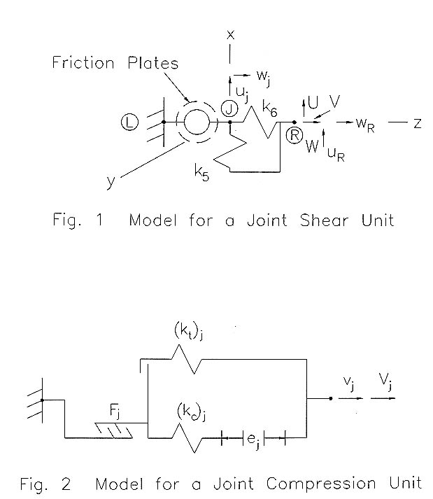
Basic, Joint Shear Unit
Referring to Figure 1 the basic, joint shear unit is modeled as a point, i.e. forces and couples are independent. It behaves as a rigid body with respect to the x-component of rotation and y-component of displacement. It resists the x-component of displacement in a complex manner as explained subsequently. The shear unit has no inertial properties. The goal of the following development is to derive instantaneous, elemental structural damping matrices by creating an algorithm obeying the elementary laws of Coulomb friction for contacting surfaces.
Shear Unit Kinematics. The motion of points J (Fig. 1) and R in the x-z plane (four degrees of freedom) is of interest. It is desired to represent the shear unit behavior with a constant total of two degrees-of-freedom in the x-z plane. This is accomplished by imposing one of the two constraints on the incremental motion: constraining either points J and L or points J and R to zero relative, incremental motion.
Shear Unit Resistance. The friction plates and spring element is in series (Fig.1).
Thus:
when there is no slipping, or

when there is friction-resisted slipping, (condition 2) or
![]()
when slipping occurs with no frictional resistance (condition 3).
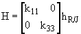
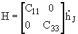
Where H is the applied force array in x-z direction. U, V and W are the applied forces in the x-, y-, and z-directions respectively. k11 and k33 are stiffness coefficients, and C11 and C33 are damping coefficients. UR and WR are the x- and z-direction deflections respectively of point 'R'.
Shear Unit Operating Conditions. The basic joint shear unit must be in one of three conditions. In condition "1", the normal force in the friction plates is compressive, and the relative velocity between the plates is zero, and the magnitude of the shear force between the plates is less than the static friction limit. The response of the shear unit is determined by the two linear springs. Condition "2" is the condition of slipping between the friction plates with Coulomb friction resisting the relative motion. For a compressive normal force in the plates it is defined by either of two sets of criteria: the plates have zero relative velocity and the static friction limit of the plates is exceeded or the relative velocity of the shear plates is nonzero. The shear unit resistance, determined by the friction plates, has a magnitude of the compressive normal force and is opposite the direction of the relative velocity while the incremental resistance represents the effect of the changing direction of the frictional resistance. Condition "3" is the condition of slipping between the friction plates with no resistance.
Transitions between Operating Conditions. Point 'J' is strictly an internal node. In order to avoid an abrupt change in the direction of the resisting force when transitions are made from conditions "2" or "3" back to condition "1" the following adjustments to the spring element total displacement are made when a transition is detected. When a transition from condition "2" to condition "1" is detected the total spring deflections are reset according to the following equation:

where k5 and k6 are the spring element spring constants. When a transition from condition "3" to condition "1" is detected the total spring deflections are reset according to the following equation:
![]()
Essentially, the spring elements are assumed to instantly adjust to the force in the shear unit. The total instantaneous slip across the plates is the total displacement of the unit minus the extension of the springs.
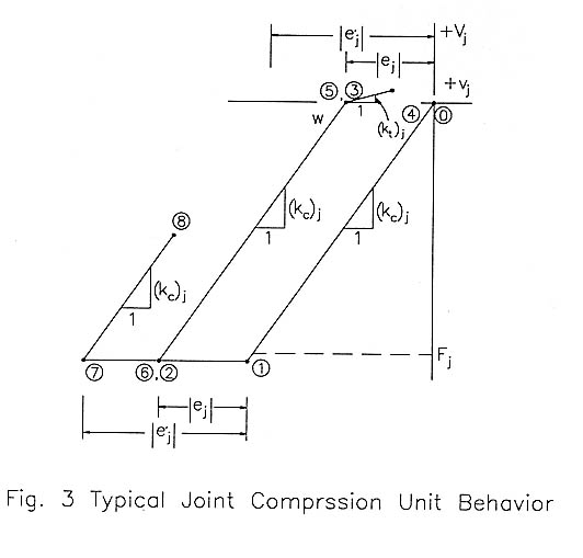
Basic, Joint Compression Unit
Referring to Figure 2, the basic, joint compression unit is modeled as a point. It is a two-force element capable of sustaining a force only in the y-direction, in a complex manner as explained subsequently. The compression unit has no inertial properties. Figure 2 represents the j'th joint compression unit as an internal gap, ej, (representing the degradation of the joint material and defined as negative if the gap is "opened", positive if the gap is "closed"), a linear, compression spring, (kc)j, and a linear, tension spring, (kt)j (representing the strain-energy-storage capacity of the joint material) and a compressive force limit in the "ratcheting", friction plates, Fj (representing the non-conservative, dissipative resistance of the joint material).
Compression Unit Resistance. As the total joint behavior is modeled with several independent compression units, consider a j'th general compression unit. The following expressions in which all of resistance is supplied by the linear spring, and 3) Condition "3" is a represent the j'th compression unit instantaneous and incremental resistance respectively:
![]()
where, Vj is the applied force, ![]() is the stiffness for the i'th operating region, vj is the total unit relative extension and
is the stiffness for the i'th operating region, vj is the total unit relative extension and ![]() is the "fixed-end" resistance for the i'th operating region.
is the "fixed-end" resistance for the i'th operating region.
Compression Unit Operating Conditions. There are three operating conditions: 1) Condition "1" is a no-contact condition. The boundary point defining this region is variable and may be adjusted during a dynamic analysis, 2) Condition "2" is an elastic-deformation slipping condition: the joint material is modeled as removing energy from the system through some non-conservative process, e.g. friction or plastic deformation.
Transitions Between Operating Conditions of the Basic Compression Unit. The internal gap for the j'th unit, ej, is reset to the following value when a transition from condition "3" to condition "2" occurs during the dynamic analysis:
![]() (7)
(7)
where ej is the new internal gap value, vj is the current unit extension, Vj is the current unit resistance and kj is the linear spring stiffness. This allows for a gap to develop.
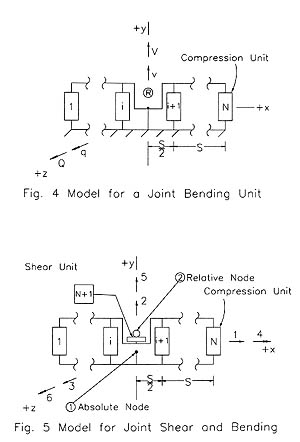
An Example Compression Unit Path in the Force-Extension Plane. Figure 3 is a graphic representation of a typical trajectory of the j'th compression unit of a joint. Initially, the internal gap, ej, is zero and the initial extension is zero; the material is in condition "2" at point '0'. The unit is in condition "2" as the spring is compressed in going from points '0' to '1'. At point '1' the limiting force, Fj, is reached and the unit is in condition "3" during displacement from point '1' to '2'. At point '2', the velocity reverses and the unit is in condition "2" during the displacement from points '2' to '3'. At point '2' the internal gap has been reset to -|ej|. At point '3' the unit returns to condition "1" and is in condition "1" as it displaces from points '3' to '4'. At point '4' the velocity reverses and the unit remains in condition "2" as it displaces from points '5' to '6'. At point '6' the limiting, force, Fj, is again reached and the units is in condition "3" during displacement from points '6' to '7'. At point '7', the velocity reverses and the unit is in condition "2" during displacement from point '7' to '8'. At point '7' the internal gap is reset to -|ej|. The unit is expected to overshoot Fj at points '1' and '6'.
Joint Element with Shear and Compression Units
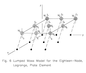
Figure 5 is a schematic of a joint, showing a single shear unit in series with a set of N compression units assembled in parallel as shown in Figure 4. The joint is modeled as having no geometrical dimensions except the compression unit spacing, S, which allows the joint to resist the z-component of a couple.
Stability and Constraints. The joint model does not provide resistance to the x- and y-components of relative rotation across the joint. Normally, when a complete system model is assembled, these displacements are constrained to remain zero.
Calculating the Compression Unit Spacing. As shown in Figure 4, the joint capacity to resist motion in the y-direction and a couple about the z-axis is provided by N, equally spaced, compression units. For the following derivation the region of a physical system being modeled, is conceived of as a rectangular contact area in the x-z plane and the material enclosed within the box generated by translating this rectangle one half thickness in the positive y-direction and one-half thickness in the negative y-direction. Each compression unit is assumed to represent an equal area.
Compression units '1' through 'N' are all assumed to be in condition "2", i.e. with linear springs engaged. The normal strain in the material is assumed to be proportional to the distance from the neutral axis of the area in the x-z plane, xna, and the normal stress is assumed to be proportional to the normal strain. The unit spacing is calculated to insure the equality of the total resisting moment of the 'N' compression units and the rectangular area of the joint material about the neutral axis as expressed in the following equation:
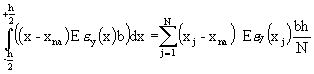 (8)
(8)
where, h is the joint material thickness or depth (x-direction dimension), xna is the x-coordinate of the neutral axis, E is Young's modulus of the joint material, ![]() is the y-directional normal strain in the material as a function only of 'x' and b is the width (z-direction dimension of the joint material).
is the y-directional normal strain in the material as a function only of 'x' and b is the width (z-direction dimension of the joint material).
This method has been used to model the deformation of ring structures under dynamic loads (Singhal, 1969); a complete analysis is given in this reference. The spacing is then given by the following equation,
![]()
where, S is the compression unit spacing and h is the joint material thickness or depth.
Defining Collision at a Joint Element
Collision is first defined for a joint, compression sub-element and then the former definition is used to define collision for an entire joint element. Collision at a joint compression sub-element occurs when simultaneously the sub-element goes from a tension condition (condition "1") to a compression or slipping condition (conditions "2" or "3") and the relative velocity across the sub-element is negative, i.e. produces further compression. The contact point for calculating the effect of the collision is at the centroid of the locations of the colliding sub-elements.
Joint Pre-Displacements
The just discussed scheme for modeling nonlinear joint behavior easily accommodates joint element pre-displacements. A pre-displacement is a normal deflection, along the joint y-axis, or a rotation about the joint x-axis displacing the element from its undistorted configurations before insertion into the structural model. These pre-displacements are added to any calculated displacements in determining the joint element state and their effect is calculated during an iterative solution for the finite-element model's static configuration.
JOINTS WITHIN THICK BEAMS, AND THICK PLATES
A critical feature of the systems chosen for analysis is that the depth or thickness of the systems' components exceeds one-tenth their lengths, requiring the consideration of shearing deformation. It is also desirable to have models capable of representing rigid-body displacements and the inertial resistance of material rotating about the element midlines or mid-planes.
If the joint-element stiffness matrix is defined in terms of absolute reference system, then the magnitudes of the joint-element-stiffness matrix entries are much larger than the magnitudes of elements in the stiffness matrices corresponding to bulk of the structure. This results from attempting to model with the joint element a small, compact volume of material relative to the extended dimensions of the elements modeling the remaining structure. Consequently, an ill-conditioned system, stiffness matrix is generated. If the system configuration is represented with both absolute, generalized displacements and relative general displacements, then this problem is avoided. Transforming an all-absolute set of generalized displacements to a mixed set of absolute and relative, generalized displacements is a common procedure in analyzing general, mechanical systems.
Figure 6 is a schematic depiction of the lumped inertial properties; the smaller filled circles are the nine absolute nodes each shown connected by a broken line to a point mass and a uniform bar located at a relative node.
Thick Beam Finite-Element
The exact, stiffness matrix developed for thick beam with shear deformation, is used in the segmented-arch analyses.
When a crack or construction-related joint has been opened and later closes, the material on either side of the contracting surfaces will not have zero relative velocity at the instant of contact. This is treated as an eccentric impact of two rigid bodies.
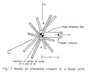
Eccentric, Interplate Impact at a Joint, for Skewed Mass Elements Meeting at a Joint
Figure 7 depicts the model of the impact process at a joint element. The point masses of bodies A and B are the scalar sums of the point masses associated with the plate elements contacting the joint, transformed into the joint coordinate system.
Joint Constraint, Skew Case. Interaction at the contact point is assumed frictionless. This is expressed by the following constraint equations enforced during the impact period:
![]() (10)
(10)
where ![]() and
and ![]() , y-direction velocities of points I and J respectively, are equal during impact.
, y-direction velocities of points I and J respectively, are equal during impact.
At all times points I and J are rigidly connected to bodies A and B respectively by massless rods. This is expressed by the following rigid-body constraints enforced at all times
![]() (11)
(11)
![]() (12)
(12)
where ![]() and
and ![]() are the y-components of velocity of the centers of mass of bodies A and B respectively,
are the y-components of velocity of the centers of mass of bodies A and B respectively, ![]() A and
A and ![]() B are the z-components of the angular velocities of bodies A and B respectively, and "a" is the impact offset.
B are the z-components of the angular velocities of bodies A and B respectively, and "a" is the impact offset.
The x-direction and y-direction components of the angular velocity of body B relative to body A are constrained to zero. This is expressed by the following constraints:
![]() (13)
(13)
where, ![]() A and
A and ![]() A are the x and y components respectively of the angular velocity of body A, and
A are the x and y components respectively of the angular velocity of body A, and ![]() B and
B and ![]() B are the x and y components respectively of the angular velocity of body B. The x and z components of the velocities of the centers of mass of bodies A and B are unchanged by the impact. Then the values after impact must be determined by the dynamics of the impact
B are the x and y components respectively of the angular velocity of body B. The x and z components of the velocities of the centers of mass of bodies A and B are unchanged by the impact. Then the values after impact must be determined by the dynamics of the impact
Impulse and Momentum, Skew Case. It is assumed that the only forces acting during impact are the contact forces at points I and J. These forces are parallel to the y-axis. Impact is assumed completely elastic. Considering the two bodies as a single system, the system linear and angular momentum must be conserved during impact. The equality of the total linear impulse and change in linear momentum, and the equality of total angular impulse and change in angular momentum, assuming elastic, frictionless contact, are applied to each body.
Conservation of Kinetic Energy, Skew Case. To completely define elastic impact the conservation of kinetic energy principle is applied to the two bodies as a single system. The terms involving the x and z components of velocity of the bodies have been deleted from the energy expression as they are unchanged by the impact.
Conditions on the Solution of the Impact Equations Skew Case. Since the energy equation is quadratic, two distinct solutions exist for these impact equations; one corresponding to repulsive interaction forces and a second corresponding to attractive interaction forces.
Eccentric, Interplate Impact at a Joint, Coplanar Mass Elements Meeting at the Joint. When all of the plates associated with a joint are coplanar in the joint x-z plane the impact problem may be modeled as the eccentric impact of two coplanar lamella. In this case, all the products of inertia are zero. The point masses of bodies A and B are the scalar sums of the point masses associated with the plate elements contacting the joint. The moments of inertia of A and B are the sums of the moments of inertia associated with the plate elements contacting the joint coordinate system.
Eccentric Impact Equations
The eccentric impact equations may be applied directly to a joint in a collision state. The constraints for the relative node of the joint must match those assumed in the impact equations' derivation. Applying the assumption that only impact related forces need be considered during the impact process the system damping and elastic generalized force vectors are ignored. The appropriate impact equations are applied in the joint element coordinate system to calculate the final, linear and angular velocities in the joint system. Finally the final linear and angular velocities are transformed back into the local, nodal coordinate system and inserted into the proper positions in the system, velocity vector.
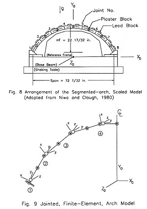
An Experimental Study of a Segmented-Arch, Scaled Model
Niwa and Clough (1980, 1982) carried out a series of experiments on a segmented arch constructed of seven rectangular blocks cast of a specially formulated mixture of water, celite, sand, lead and plaster. The properties of the formulation used in these experiments were carefully tailored so the response of the model to the shake table accelerations it was subjected to could be scaled to predict the response of a full-size structure. The blocks were carefully assembled on a shake table to remain erect under the influence of gravity without applying adhesive to the contacting surfaces. Radial and tangential, dynamic, displacements were recorded at the center of each block. Relative, dynamic, joint displacements were recorded at the upper edge of each joint. Dynamic normal strains were measured at three points in each block on the convex, upstream, surface along a line at the block mid-width; at mid-length, and at one inch from each end. To indicate joint opening contact sensors were installed at the upper and lower joint edges. In order to provide a model size that could be constructed and tested conveniently on a shake table that produces model strains equal to those of the full-size prototype, ratios of critical variables were selected so the ratio is unity for unit weight, Poisson's ratio, strain and acceleration. Tests were conducted with vertical (y-direction) base acceleration only, horizontal (x-direction) acceleration only and with combinations of vertical and horizontal base accelerations. The authors conclude that for the most intense vertical-acceleration-only test, 0.226g-peak acceleration, the effect of joint non-linearity is negligible. They also conclude that for the least intense horizontal-acceleration-only test, 0.039g peak acceleration, the deflections and strains are affected by joint non-linearity. The clearest indicator of joint non-linearity is a decrease in peak tensile strains on block surfaces near a joint edge at which block-to-block contact has been lost.
Description of the Experimental and Numerical Models
The experimental model and results of Niwa and Clough (1980, 1982) were chosen to test the joint model and numerical procedures. A 1:150 scale model was used. A diagram of the experimental model is given in Figure 8 and a schematic for its mathematical representation is given in Figure 9. The dimensions of the blocks making up the experimental model are 9 inch (22.9 cm) wide by 3-3/16 inch (8.1 cm) thick by 13-5/16 inch (33.8 cm) long with material properties given on Table 1.
Table 1 Mechanical properties of the scaled, model material
|
E |
|
|
Unit mass |
|
|
27.7 x 10³ (psi) |
26.5 (psi) |
2.81 (psi) |
74.9 (lbm) |
0.17 |
|
191 (MPa) |
0.183 (MPa) |
0.019 (MPa) |
1200 (kg/m3) |
Finite-Element Model Geometry
Finite-element models of the model tested by Niwa and Clough (1980, 1982) have been created using the shear beam element and the discrete, nonlinear, joint element developed in this paper. One model, referred to as the jointed model, consists of fourteen shear-beam elements arrayed along the mid-thickness plane centerlines as indicated by the broken line through the arch blocks of Figure 8. Eight joint elements are inserted at two-beam-element intervals and at the abutments. Only relative rotation about the ZO-axis is allowed at the joint, relative nodes. Model geometry, constraints and local coordinate systems are shown in Figure 9. The other model, referred to as the unjointed model, is identical to the jointed model, but constraining the joint, relative nodes to zero displacements eliminates joints. In Figure 9 the following conventions are followed: an open circle represents a relative node; a filled circle represents an absolute node; an open circle surrounding a filled circle indicates a relative node constrained to move with the surrounded absolute node; an open circle touching a filled circle or touching an open circle containing a filled circle indicates the absolute node used as the original relative reference node. The generalized displacements of absolute nodes are specified in a coordinate system moving with the foundation. The generalized displacements of each relative node are specified as relative to a particular absolute node, the reference node. A joint element is inserted at each of the eight locations where a relative node is free to rotate.
Influence of the Joint Sub-element Properties on System Response
The beam elements' thickness and length are the same as the blocks in the experimental model. Damping is modeled by the Rayleigh method; the Rayleigh coefficients for the system mass and stiffness matrices are for 3% damping at the two experimentally determined symmetric modes reported by Niwa and Clough with angular frequencies of 75.4 radians/sec and 151 radians/sec. Comparing the computed value for the dynamic, vertical deflection of the arch center-line node to the corresponding value determined experimentally, at 0.12 sec; the experimentally-determined deflection is 0.00300 in (0.00762 cm) for a 0.3g peak acceleration and the computed deflection is 1.91 times as large as 0.00572 inches (0.01453 cm).
Comparing the computed value for the dynamic, vertical deflection of the arch centerline node to the corresponding value determined experimentally, at 0.12 sec; the computed deflection is 0.00622 inches (0.01580 cm), i.e., 2.07 times the experimentally determined deflection of 0.00300 inches (0.00762 cm). The computed peak, dynamic deflection for the jointed, finite-element model is 8.4% larger than the computed, peak, dynamic deflection for the unjointed, finite-element model. These results are summarized in Table 2. The angular frequencies of these modes were calculated to be 87.9 radians/sec and 178 radians/sec.
Table 2 Summary of Experimental and Computed Peak, Dynamic Deflections for
Segmented Arch
|
Computed Deflection, Unjointed Model Experimental Deflection |
1.91 |
|
Computed Deflection, Jointed Model Experimental Deflection |
2.07 |
|
Computed Deflection, Jointed Model Computed Deflection, Unjointed Model |
1.08 |
Plate Model Geometry and Material Properties
Each model consists of twenty, square, thick-plate elements arranged in four rows of five elements. Each plate element is uniformly 3-1/16 inch (8.10 cm) thick and 6-21/32 inch (16.91 cm) square. Their material properties are the same as used for the shear-beam elements of the arch, finite-element model. Each thick-plate element is the eighteen-node, element with nine absolute-relative node pairs. Each joint element is represented with fifty compression sub-elements and a shear sub-element.
Table 3 Joint Thickness and Friction
Coefficients, for the Plate Models
|
t |
|
|
|
2.5 (10-5) in. (6.35(10-5)cm) |
.20 |
.18 |
Results for the Continuous Finite-Element, Plate Model
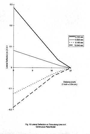
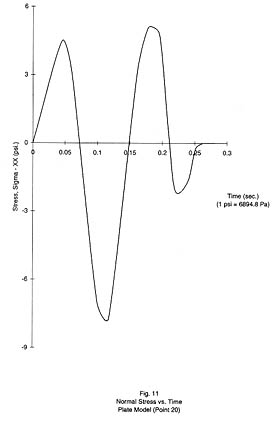
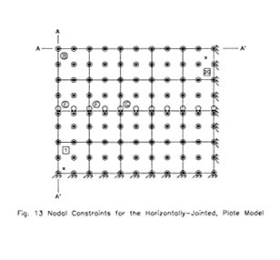
Figures 10 through 12 illustrate the response of the continuous-plate, finite-element model at the 0.3g peak foundation acceleration. Figure 10 shows the absolute lateral deflection (1in. = 2.54 cm) at the free edge on the centerline. Figure 11 shows the total, normal stress (1 psi = 6895 Pa) on the global Y-Z plane in the front surface plane at the Gauss point indicated in plate point 20, as shown in Figure 13.
Results for the Horizontally-Jointed Finite-Element, Plate Model
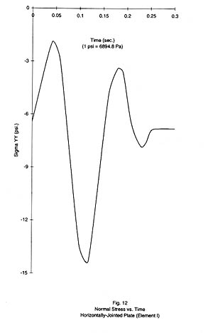
The primary contrast between the horizontally jointed, plate model and the continuous plate model is the slipping against Coulomb friction at the joint elements along the horizontal joint line. The shear stiffness in the joint elements is large enough that the response of the horizontally jointed model does not differ from the continuous plate response until slipping begins in the joint elements. The dynamic shear stress first breaks the frictional bond at nodes (Figure 13) 'E' through 'F' at 0.110 sec just before the peak negative base acceleration reaches 0.117 sec. By 0.165 sec slipping is occurring at node 'G' and ultimately all of the joint elements slip. The relative deflection before slipping occurs is negligible compared to the relative deflection due to slipping. After the foundation acceleration returns to zero at 0.283 sec the velocities of the free relative nodes along the joint line quickly return to zero and a permanent displacement of these nodes relative to their reference nodes remains as shown for node 'E'. The effect of this permanent deflection due to slip is evident in the post-foundation-acceleration, elastic deflection and the decrease in negative peak deflection at 0.180 sec to 44% of the continuous-plate value at absolute node 'A'. In plate element I (Figure 12) the peak dynamic stress values at 0.180 sec and 0.225 sec are decreased to 58% and 67% of their respective continuous-plate values and a residual stress of -7.0psi (-4.82 KPa) in addition to the gravity stress remains.
Results for the Vertically-Jointed Finite-Element, Plate Model
The primary contrasts between the vertically jointed plate model and the continuous-plate model are the result of slipping in the compression sub-elements. This slipping produces a permanent rotation in joint elements.
Horizontally- and Vertically- Jointed Finite-Element, Plate Model
The response of this model is influenced both by slipping against Coulomb friction at the joint elements along the horizontal joint line and slipping in the compression sub-elements of some of the joint elements along the vertical joint lines. There is evidence of the interaction of these two processes. The shear stiffness in the horizontal-joint-line elements is large enough that the response is not affected until slipping occurs.
CONCLUSIONS
A discrete, joint element, which incorporates several novel capabilities, has been developed and applied to the dynamic analysis of localized discontinuities in a segmented arch and a thick, flat plate. This joint element models nonlinear material behavior, accounting for different tensile and compressive stiffness, perfectly plastic slipping or yielding, and hysteresis. Coulomb friction at the joint is accounted for. Collision at a joint is incorporated by using the eccentric impact equations for the transfer of momentum and kinetic energy during the impact of two rigid bodies and applying them to a lumped mass representation of a structural system's inertial properties. A computer program has been developed for solving the initial static response accounting for joint, material non-linearity and later calculating the dynamic solution of the system. Iteration methods are used. Iteration continues until the joint element's calculated forces and deflections are consistent with the joint element's material properties used to generate the system stiffness matrix. For the solution of the system equations of motion, the program uses the Newmark Beta method. If at any step in the solution, the Newmark Beta method fails, an attempt is made to successfully complete the step with a Runge-Kutta method. When successful, it is preferable to take a solution step with a Newmark Beta method as this uses much less computational time than the Runge-Kutta method. Normally trouble is encountered with the Newmark Beta method when a change in joint element mechanical properties forces the system stiffness matrix to become ill conditioned.
This joint element has been incorporated into a finite-element, model of an actual scale-model, segmented arch which has been tested on a shake table by previous researches and the calculated response compared to the experimental results reported in the literature. This joint element has also been incorporated into finite-element, models of a thick plate fixed on three edges, free on the fourth edge and subjected to lateral base accelerations. Models were generated with no joints, with a single joint line, parallel to the free edge, exhibiting Coulomb friction; with six, equally-spaced, joint lines parallel to the opposing fixed edges, exhibiting nonlinear material behavior and interplate collisions; and with a combination of the previous two sets of joint lines. The results of these analyses are presented and the effects of the joint lines on the model behavior are discussed.
It is concluded that Coulomb friction, material non-linearities and collisions can be successfully incorporated into a time-domain solution of a finite-element, structural model and that the resulting analyses can be used to assess the effects of these types of mechanical behavior on the system response.
REFERENCES
ADINA Engineering, 1984, "Automatic Dynamic Incremental Non-Linear Analysis," report AE 84-1, ADINA Engineering, Watertown, MA.
Bathe, K.J., Wilson, E. and Peterson, F.E., 1973, "SAP IV, a Structural Analysis Program for Static and Dynamic Response of Linear Systems," Report No. 73-11, EERC, Univ. Cal., Berkeley, CA.
Boggs, H.L. and Mays, J.R. 1987, "Effects of Vertical Construction Joints on the Dynamic Response of Arch Dams," Joint Meeting, NSBIR 87-3540, U.S. Dept. of Comm., N.B.S., Wash., D.C.
Fenves, G. and Chopra, A.K., 1984, "Earthquake Analysis and response of concrete Gravity Dams," Report No. UCB/EERC-85/07, EERC, U. Cal., Berkeley, CA.
Hall, J.F. and Dowling, M.J., 1985, "Response of Jointed Arches to Earthquake Excitation," Earthquake Engr. And Structural Dynamics, 13 No. 6, Nov.-Dec., 779-798.
Niwa, A. And Clough, R.W., 1980, "Shaking Table Research on Concrete Dam Models," Report No. UCB/EERC-801/05, EERC, U. Cal., Berkeley, CA.
Niwa, A. and Clough, R.W., 1982, "Nonlinear Response of Arch Dams," Earthquake Engr. And Structural Dynamics, 10, No. 2, Mar.-Apr., 267-281.
Nuss, L.K. and Singhal, A.C., 1987, "Static and Dynamic Stability at Stewart Mountain Dam," Technical Memorandum, SM-220-01-86, U.S. Bureau of Reclamation, Denver, CO.
Persson, V.H. and Ahmad, R., 1987, "Criteria for Safe Dam Performance in California," China-U.S. Workshop on Earthquake Behavior of Arch Dams, Tsinghua U., Beijing.
Rea, D., Liaw, C.Y., and Chopra, A.K., 1975, "Mathematical Models for the Dynamic Analysis of concrete Gravity Dams," Earthquake Engr. And Structural Dynamics, 3, 249-259.
Roehm, L.H., 1971, "Comparison of computed and Measured Dynamic Response of Monticello Dam," Report No. REC-ERC-71-45, U.S. Bureau of Reclamation, Denver, CO.
Row, D. And Schricker, V., 1984, "Seismic Analysis of Structures with Localized Nonlinearities," Proceedings of the Eighth World Conference on Earthquake Engr., San Francisco, CA.
Scott, G.C. and Von Thun, J.L., 1987, "Evaluation of Arch Dam Foundations of Earthquake Loading," China-U.S. Workshop on Earthquake Behavior of Arch Dams, Tsinghua U., Beijing.
Singhal, A.C., 1969, "Nonlinear Dynamic Response of Bonded and Unbonded Rings Under High Intensity Blasts," J. Indian Institute of Engineers, 50, September 1-11.
Singhal, A.C., and Nuss, L.K., 1986, "Dynamic Earthquake Analysis of Morrow Point Dam Structures," Tech. Memorandum, MP-221-1, Dam and Waterways design, U.S. Bureau of Reclamation, Denver, CO.
Singhal, A.C., 1986, "Structural Engineering Issues-Dynamic Analysis of Concrete Structures of Kortes Dam," Tech. Memorandum, KD-221-1, Dam and Waterways design, U.S. Bureau of Reclamation, Denver, CO.
Singhal, A.C., 1987, "Evaluation of the Effects of Water Compressibility on Seismic Behavior of Dams," Tech. Memorandum, SM-221-1, Dam and Waterways design, U.S. Bureau of Reclamation, Denver, CO.
Singhal, A.C., 1991, "Comparison of Computer Codes for Seismic Analysis of Dams," Computers and Structures," 38(1), 107-112.
Singhal, A.C., and Nuss, L.K., 1991, "Cable Anchoring of Deteriorated Arch Dam," J. of Performance of Constructed Facilities, ASCE, 5 (1), Feb. 19-36.
Tarbox, G.S., Dreher, K.J., and Carpenter, L.R., 1979, "Seismic Analysis of Concrete Dams," Proceedings of the 13th International Congress on Large Dams, 2, Q.51, R.11, New Delhi.
U.S. Department of the Interior, 1971, "Forced Vibration Tests of Morrow Point Dam," J.G. Bouwkamp, June, 1971, Contract No. 14-06-D-6785.