Multiple Linear Regression - Examples
The purpose of this example is to demonstrate required computations for parameter estimation with a small scale multiple regression example. Those computations will be compared to results from Microsoft Excel regression output. Please complete all parts of the example. Note that some values you obtain may be different from values obtained using the software because of rounding.
This example covers three cases of multiple linear regression using a data set of four observations. In practice this number of observations would be considered to be unacceptably small. The reason for a small data set is to keep the computations simple and transparent. Once you know how the modeling approach works in small cases you will be confident in using this approach even as the data sets become large.
The cases are developed in two phases, first, by constructing tables for step-by-step computations, and secondly, running the Microsoft Excel Regression Analysis Tool on the same data. The objective is to demonstrate
- how perfect regression can occur, and how to see it from the numbers,
- how multiple linear regression models can be easily developed even without specialized software,
- some pitfalls of multiple regression,... numbers look good, but ...
- how step-by step computations compare to Microsoft Excel output, and how output values can easily be verified.
Note: Please keep in mind that all statements made here with respect to multiple linear regression are also valid with polynomial- and non-linear regression models later.
Let's look at the three cases.
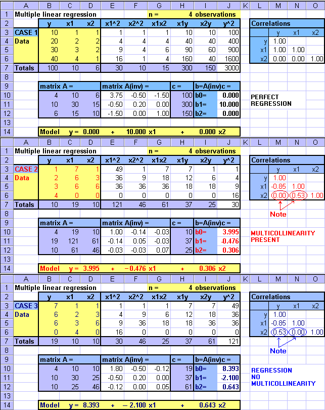
The first part of the figure and animation below show the data in the first three columns: the first column gives the four y values followed by x1 values in the second column and x2 values in the third column. These data columns are followed by columns of intermediate computations: values of x1 squared, values of x2 squared, values of x1 multiplied by x2, values of x1 multiplied by y, values of x2 multiplied by y, and values of y squared. The column totals are used to develop the matrices A and c of the system of linear equations Ab=c.
Below the data table are the matrix tables for A, A-1, c and the matrix product A-1c = b. The matrix (or vector) b is then the set of parameter values b0, b1, and b2. Please note that the gray shaded matrix A and c numbers come from the gray shaded column totals of the intermediate computations.
The multiple regression model is then given below the matrices.
In addition, a correlation table is presented to the right of intermediate computations. Please observe the correlations between the variables, and refer to earlier discussion about regression model assumptions.
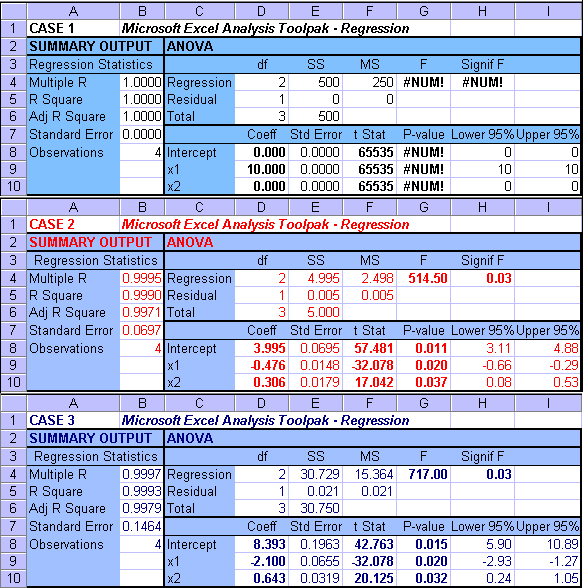
The second part of the figure gives the Microsoft Excel Regression Analysis Tool output for the same cases respectively. Please note the familiar layout of the ANOVA (Analysis of Variance) table. Information in that ANOVA table corresponds to the table given in the section - Model Testing for multiple linear regression. When in doubt, please look there for some model testing details. The ANOVA table summarizes the information for the overall regression significance test (F-test). The table below that gives the parameter (b0, b1, b2) estimates in column titled Coeff, as well as information for the parameter significance tests (t-tests).
The cases are presented as an animation. Please observe how the data changes, and how that affects all computations and results. If you want to capture the cases separately for closer study and analysis, please use PrintScreen from your keyboard and then save the image in a file.


Case 1: Perfect Regression
In this case, when the data values of x1 increase then
the values of y increase linearly and proportionally. The values of
x2 first increase and then decrease. The least
squares estimation comes with a perfect relationship between y
and x1 with b1=10, and
b0=b2=0. When you substitute x1
values to the model  = 10x1
you obtain the y data values exactly. Hence, there is no error. Also,
the multiple linear regression model collapses to a simple linear regression model.
Note: The MS Excel function MINVERSE is used to find the matrix inverse A(inv) of matrix A. The matrix (or vector) b=A(inv)c=A-1c is found using the matrix product function of MS Excel called MMULT. Please play with these and other functions of the software, they might become quite helpful later.
In the table of correlations you can see that there is a perfect correlation between x1 and y. However, there is no correlation between x2 and y, and between x1 and x2.
Please see how Excel handles this situation. Because there is no error, the standard errors and residuals (SSE) are zero, and hence the F- and t-statistics cannot be calculated (cannot divide by zero). (see #NUM in the output table). This whole case is practically not very meaningful, but it demonstrates an extreme situation.
Case 2: Regression with Multicollinearity
In this case, when the data values of x1 decrease, the values of y increase linearly and proportionally. The values of x2 first increase and then decrease with the majority of values showing an increasing pattern. The table expansion computations and the MS Excel Regression come up with identical parameter estimates. As expected, the sign of b1 = -0.476 is negative suggesting that the values of y and x1 move into opposite direction (i.e. when values of one variable increase in the data the values of the other decrease and vice versa). Also as expected, the sign of b2 = +0.306 is positive suggesting that the values of y and x2 tend to move into the same direction (i.e. when values of one variable increase in the data the values of the other also increase and vice versa).
Note: The MS Excel function MINVERSE is used to find the matrix inverse A(inv) of matrix A. The matrix (or vector) b=A(inv)c=A-1c is found using the matrix product function of MS Excel called MMULT. Please play with these and other functions of the software, they might become quite helpful later.
The standard error is not zero, and hence SSE is not zero suggesting that the data points deviate from the model line (plane). Also, the parameter standard errors are not zero. Hence, the F- and t-statistics can be determined and the tests can be conducted as usual.
The Fcalc = 514.50 and Signif F = 0.03 < 0.05 suggest that the overall regression is significant.
The tcalc values, and the corresponding P-values (all < 0.05) suggest that all parameters b0, b1 and b2 are significant. This is also supported by the confidence intervals (no confidence interval contains zero).
All tests look good, so the model must be good!?!! WAIT!!! OK, go and get a cup of coffee or tea or something. ... Where are you going!!
Look at the correlations. There may be a problem. The correlation coefficient between values of x2 and y is zero. Changes in the values of an independent variable (here x2) were supposed to affect (or explain) changes in the values of the dependent variable (here y). But we determined that parameter b2 is significant, and MS Excel output did not suggest any problems. This is not a good sign, ... is there an explanation. Take a look at the correlation coefficients again. There appears to be a quite strong (r=0.53) relationship between the independent variables x1 and x2. Please recall that in multiple linear regression we assume that the independent variables are independent of each other. If variables are independent then there should be no association between them, and consequently the correlation coefficient should be zero. The presence of association between independent variables is called multicollinearity. Some multicollinearity is likely to be present in most practical multiple regression cases.
Note: Two variables can be completely multicollinear, and hence one can be shown to be a linear combination of the other. One of the two completely multicollinear variables is redundant and should be eliminated. The presence of highly multicollinear variables may affect model parameter estimates significantly. This can cause unwanted bias in the model. One approach to avoid or reduce multicollinearity is to use stepwise regression.
Case 3: Multiple Regression
In this case, when the data values of x1 increase linearly and proportionally, the values of y decrease. The values of x2 first increase and then decrease with the majority of values increasing. The table expansion computations and the MS Excel Regression come up with identical parameter estimates. As expected, the sign of b1 = -2.100 is negative suggesting that the values of y and x1 move into opposite direction (i.e. when values of one variable increase in the data the values of the other decrease and vice versa). Also as expected, the sign of b2 = +0.643 is positive suggesting that the values of y and x2 tend to move into the same direction (i.e. when values of one variable increase in the data the values of the other also increase and vice versa).
Note: The MS Excel function MINVERSE is used to find the matrix inverse A(inv) of matrix A. The matrix (or vector) b=A(inv)c=A-1c is found using the matrix product function of MS Excel called MMULT. Please play with these and other functions of the software, they might become quite helpful later.
The standard error is not zero, and hence SSE is not zero suggesting that the data points deviate from the model line (plane). Also, the parameter standard errors are not zero. Hence, the F- and t-statistics can be determined and the tests can be conducted as usual.
The Fcalc = 717.00 and Signif F = 0.03 < 0.05 suggest that the overall regression is significant.
The tcalc values, and the corresponding P-values (all < 0.05) suggest that all parameters b0, b1 and b2 are significant. This is also supported by the confidence intervals (no confidence interval contains zero).
Let's again look at the correlations. The correlation coefficient between the independent variables is zero, suggesting that there is no association between the variables. The correlations between each independent variable and the dependent variable suggest that a relationship may exist.
All tests look good and correlation coefficients make sense. So far, all indications are that the model is good.
Note: I strongly recommend that you repeat the step-by-step computations and create the corresponding Microsoft Excel table (with formulae). This will add confidence into regression modeling when your deal with large numbers of variables or large data sets.