Multiple Linear Regression - CASE
Household Survey
This example looks at an actual household survey and data. The purpose of the survey was to determine if household income could be predicted with reasonable accuracy from data consisting of information relating to households and heads of households. Data on the following variables were gathered:
- annual income (inc_annual) of the head of the household,
- educational level (edu_yrs) attained (in terms of number of years school completed),
- length of current employment (emp_yrs) in years,
- age (age_yrs) of the head of the household,
- household size (fam_size)in terms of number of family members, and
- size of the residence (res_size).
One hundred complete surveys were received. It was believed that the sample represented the demographic characteristics of the population of the target area quite well.
It was expected that there would be a significant relationship between the annual income and one or more of the other variables. There was no clear expectation about the relationship between income and family size. However and in particular, it was believed that, on an average, there is a positive relationship between income and
educational level,
tenure with an employer (seniority),
age, and
size of residence.
Here income is treated as the dependent variable, and all other variables are considered to be independent variables. The analysis consists of three parts
- plotting of income against each independent variable,
- graphical linear regression line fitting using MS Excel Trendline function for strongest relationships,
- multiple linear regression model development, parameter- and model testing using MS Excel Data Analysis Tools.
Note: Please keep in mind that all statements made here with respect to multiple linear regression are also valid in other regression modeling.
Scatter Plots
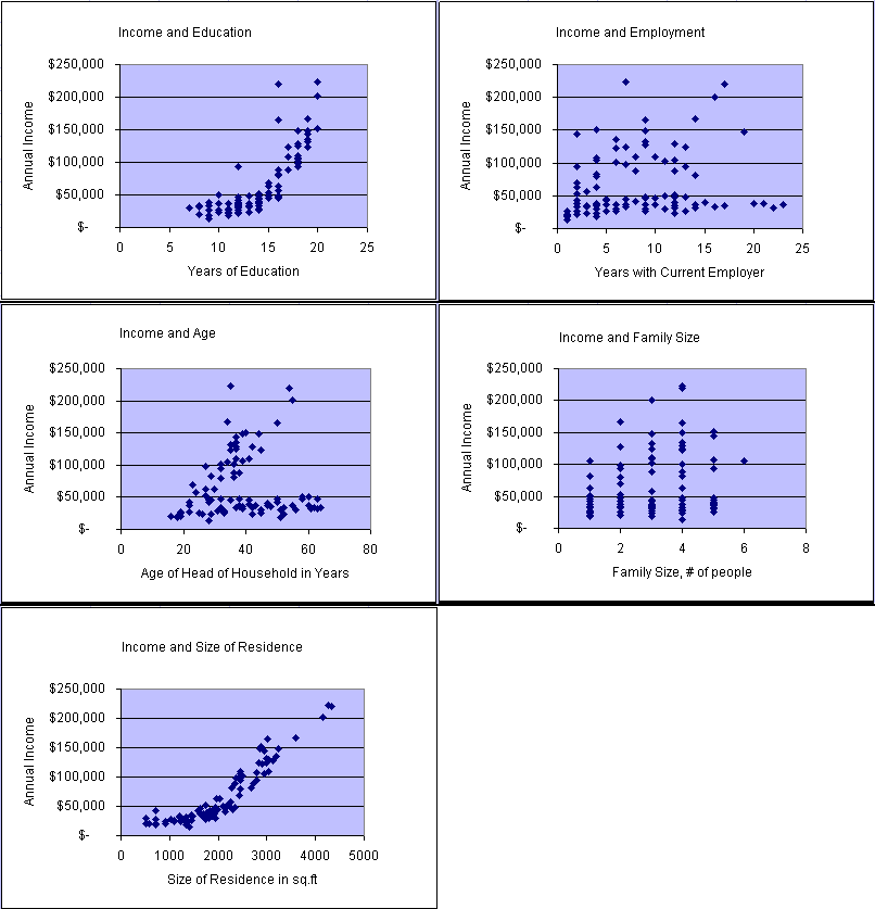
You can see from the scatter plots and animation that the patterns of data points appear to vary greatly from variable pair to variable pair. There is randomness in each plot. Two plots show a quite strong relationship: income vs. education and income vs. size of residence. However, no scatter plot appears to form a straight line. Can we go anywhere with linear models!!!
Note: In practice you should also visually study plots of each independent variable pair. Please recall the assumption that independent variables are independent of each other (i.e. no multicollinearity).
Even though we did not see any obvious linear relationships, we will go ahead and develop a multiple linear regression model for this case. However, before we do that let's develop simple linear regression models for the two strongest relationships: income vs. education and income vs. size of residence.
Simple Linear Regression Line Fitting
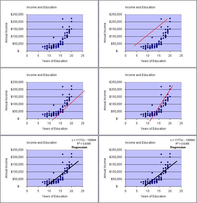
In the above animation we used the MS Excel Trendline function
to fit a simple linear regression line into the data set
to study the strength of the linear relationship between the variables
income and education. The simple linear regression
model becomes  = 11772x - 100944
with an R2 = 0.6385. This means that the model
explains about 63.85% of the variability in the data. In the
graph we can observe that the data form a distinct non-linear
pattern, which appears to start above the regression line, then fall
below the line, and finally return back above the model line. Please
keep this characteristic (scatter plot pattern) in mind when we
later test multiple regression model assumptions.
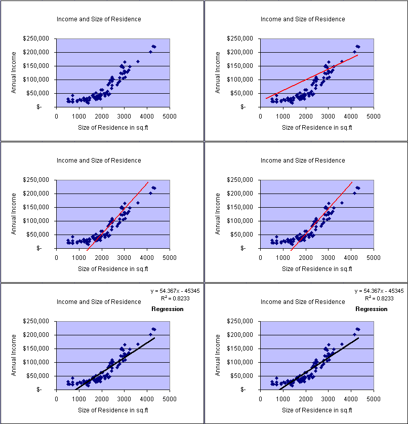
In the second animation we repeated the same process and fitted a simple
linear regression line to study the strength of the linear relationship between
the variables income and residence size. The simple linear
regression model becomes  = 54.36x - 45345 with an R2 = 0.8233. This means that
the model explains about 82.33% of the variability in the data. In the
graph we can observe that the data form a distinct non-linear
pattern, which appears to start above the regression line, then fall
below the line, and finally return back above the model line. This scatter
plot appears somewhat tighter (less variability with respect to the line)
compared to the previous model. Please keep this characteristic
(scatter plot pattern) in mind when we later test multiple
regression model assumptions.
You can see that both animations appear to result into reasonable simple linear regression models.
Regression Model Development, Parameter- and Model Testing
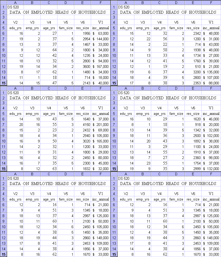
The below table gives you the data set. No need to try to copy and paste, the complete data file is available at this site. The data file is in Microsoft Excel format.
For this first model it is assumed that all dependent vs. independent variable relationships are linear, and that a multiple linear regression model fits the data best. The model development uses Microsoft Excel Analysis Tools and incorporates all variables. If one or more independent variables turn out to be non-significant, then such variables are eliminated and the model is rerun.
The first model
The table below gives the Microsoft Excel Regression output for the first model. Please study this output carefully.
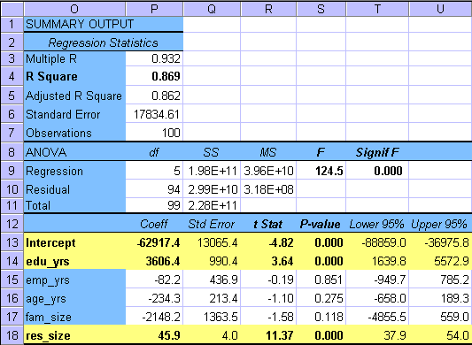
The first part of the table gives the correlation coefficient (r), coefficient of determination (r2), standard error, and the number of observations (n).
The second part of the table, titled ANOVA for Analysis of Variance contains the information for testing the overall significance of the model. This test is an F-test. The rows of the table partition the variability in the data into two groups: variability due to Regression, and variability due to error or Residual. The columns of the table give the degrees of freedom, (df), the Sums of Squares, (SS), the Mean Square, (MS) (which are the independent error variance estimates), the F-test statistic, and the Significance of F.
Test of overall regression - The Fcalc=124.5
fcritical indicates that the regression model is very
significant, i.e a significant proportion
of variability is due to the relationship between the variables. The
fcritical for df=(5,94) is obtained from
a statistical table (F-table). The same conclusion can be reached
using the Significance F-column value. This value corresponds
to a probability (i.e. area) on the tail side of the Fcalc
value. This value can be compared
to a chosen level of significance ( ). The regression is significant if the Significance
F-column value is less than the chosen
 . For example if you choose
 =0.05, then clearly
the conclusion is the same. The overall regression is significant.
Note: When you are comparing several models, the larger the F-value the more significant the model.
Parameter tests - The lower part of the table summarizes the
parameter- and parameter
test information. The parameter tests are t-tests like before.
The estimated model
parameter values for b0 = 'intercept' = -62917.4,
b1 = 'edu_yrs' = 3606.4, b2 = 'emp_yrs' =
-82.2, b3 = 'age_yrs' = -234.3,
b4 = 'fam_size' = -2148.2 and b5 =
'res_size' = 45.9 are given in
the column titled Coeff, followed by their standard errors,
t-statistics, P-values, and 95% confidence intervals.
You can use any one of the three, the t-test statistics, P-values
or confidence intervals, to conduct the tests.
From this table the multiple linear regression model becomes to
 = - 62917.4 + 3606.4 edu_yrs - 82.2 emp_yrs - 234.3 age_yrs -2148.2 fam_size
+ 45.9 res_size.
Note: If the t-test statistic falls into the critical
region, and the P-value is smaller than the chosen level of
significance  =0.05, and
the confidence interval does not include zero, then
the parameter is significant (i.e. significantly different from zero).
From the parameter t-test results one can see that the model parameters b0, b1 = 'edu_yrs' and b5 = 'res_size' are significant. This suggests that the model should be rerun without the non-significant variables 'emp_yrs', 'age_yrs', and 'fam_size' to find an improved model. This will be done next.
The second model
The table below gives the Microsoft Excel Regression output for the second model. Please study this output also very carefully.
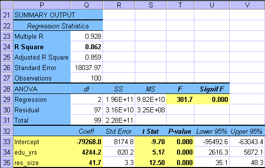
Test of overall regression - Fcalc=301.7 >
fcritical indicates
that the regression model is very significant, i.e. a significant proportion
of variability is due to the relationship between the variables. Please
note the increase in the F-value from the previous model. The
fcritical for df=(2,97) is obtained from
a statistical table (F-table). The same conclusion can be reached
using the Significance F-column value. This value can be compared to
a chosen level of significance ( ).
The regression is significant if the Significance F-column value
is less than the chosen
  .
For example if you choose
  = 0.05, then clearly the conclusion is the same as above. The
overall regression is significant.
Note: When you are comparing several models, the larger the F-value the more significant the model. In our example the second model has the larger F-value.
Parameter tests - From the model parameter t-test results
one can see that all parameters b0,
b1 = 'edu_yrs' and b5
= 'res_size' are significant. The multiple linear regression
model becomes to  = - 79268 + 4244.2 edu_yrs + 41.7 res_size.
Using the model - Now suppose, that you would like to predict
the salary of a person, who has graduated from high school (12 years
of education) and lives in a 2000 square foot house.
Substituting into the model we obtain:  = - 79268 + 4244.2 (12) + 41.7 (2000) = $55,062.
Testing the OLS - Finally, we use the residual plots to analyze visually whether or not the Ordinary Least Squares, OLS assumptions are supported. Please note that a residual plot sometimes shows the estimated errors (deviations between data points and the model line) against estimated model values, and sometimes errors are plotted against significant independent variables (here 'edu_yrs' and 'res_size'). We are looking for a random pattern of points (independency or errors) forming a horizontal band (normality of errors and constancy of error variance).
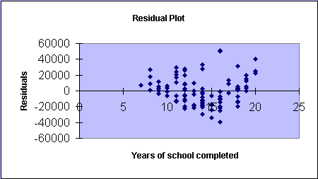
From both of the residual plots (above and below) you can see that neither scatter plot of residuals forms a horizontal random band of points of approximately equal width. Randomness appears to be present, supporting independence of errors, but the patterns do not appear to support the constancy and normality of the errors. Please recall, that we suspected something already when we studied the simple linear regression scatter plots.
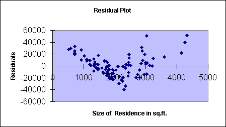
We will look at the residual plots and further model improvement in the next module.