Lecture Notes for Chapter 3

In this chapter we will take the ideas of the second law and apply them further. We first consider simple transitions like phase transitions that only involve one thing. The book derives an expression for the change in free energy of a substance as a function of temperature and pressure change. But this is a bit confusing. After all, the change in free energy is not the change in free energy of a substance, it is the change in free energy of the universe. So, how can we talk about things like molar free energies of a substance (also called the chemical potentials) if the free energy corresponds to the whole universe? We can’t have moles of the universe?? True, but we can calculate the change in free energy of the universe when a mole of something changes in some way. We are going to go through the derivation of these ideas.

The first law says:

The second law says:

Our definition of expansion-type work tells us:

putting all of this together (assuming only expansion work) we have:

OK, now a little slight of hand from partial differential equations (no, this won’t be on the exam). What this equation implies is that we can think of the total change in U in terms of two components, one the depends on the change with respect to S alone and one that depends on the change with respect to V alone (in each case holding all else constant):

By comparison, we can see that:

If it is not obvious to you why we can do this, that is not going to be a big deal in this course, but this kind of manipulation is very common in thermodynamics and other areas where one want to consider functions that depend on multiple variables.

Now, in fact we do not care too much about internal energy. That was sort of a warm up. Let’s now try this instead with Gibbs energy. Consider two phases of water, ice and liquid. The point is that as we change temperature (or pressure) the phase of water can change. How do we know which is more stable? We look at something called the molar Gibbs energy of water in the two forms and determine which form has the lowest molar Gibbs energy. To determine this, we need expressions like the ones above that tell us how the Gibbs energy depends on P and T.

So, let’s develop relationships for the Gibbs energy in analogy to those derived above for the internal energy. Recall that G=H-TS. Thus we can write down in general for dG:

but recall that

This comes from the definition of H, H=U+PV. We found a little bit ago that:

If we combine all of this together:

This again suggests that G should be a function of P and T and we can write:

comparing this to the equation above, we see that

With these two relationships, we can determine what will happen to the Gibbs free energy when either the pressure is adjusted or the temperature is changed. This is very important when we try and work through how the phase of a substance changes with pressure and temperature. At any given temperature and pressure, which phase has the lowest Gibbs free energy? These equations tell us how that energy should change with temperature and pressure and thus allow us to predict which phase (gas, liquid or solid) will have the lowest free energy. We can then generalize this to chemical reactions as well.

At this point, the book brings up the concept of molar Gibbs energy which they call G_m. This is really very similar to something the book does not bring up until later called the chemical potential. I will use that here as well, because it is easier to learn the term now rather than later (see below). The book avoids the partial differential equations I used above and sticks with the earlier relationship we derived:

dG = VdP – SdT

It then converts the Gibbs energy into the molar Gibbs energy (the Gibbs energy change per mole of the substance of interest). The equation must also be put in terms of the molar volume (the volume of a mole of the substance of interest) and the molar entropy (which we have seen before):

dG_m = V_mdP – S_mdT

Instead of explicitly using partial differential equations as we have done above, the book just states that we will hold either P or T constant and then consider the dependence of Gibbs energy on the other. For the dependence on pressure at constant temperature we have:

dG_m = V_mdP (const. T)

Thinking about this in terms of phase transitions, we can see that it makes sense. As the pressure increases, the phase with the smallest molar volume is going to be favored (because that will have the lowest increase in Gibbs energy). Generally speaking, a solid has a lower molar volume than a liquid (water being a weird exception to this rule) and liquid has a lower molar volume than gas. Thus as you increase pressure, you generally go from gas to liquid to solid, as you would expect.

Water, unlike almost all other pure substances, expands when it freezes. Arguably, this is one of the properties of water that allows for the persistence of many different lifeforms on earth because it means that ice floats. Thus lakes do not freeze solid in the winter time because the ice actually forms an insulating layer.

If you squeeze ice (even with a cold pair of pliers) the ice melts. Can you see why now?

We can also hold P constant instead of T and get:

dG_m = -S_mdT

In other words, the phase with the greatest molar entropy will decrease the most when the temperature increases. Gas obviously has the greatest entropy per mole and indeed at high temperature, it has the most negative Gibbs energy (it is the most stable phase at high temperature). However, this equation says that as you drop the temperature, gas destabilizes faster than liquid or solid, so at some point the liquid (which has an intermediate molar entropy) will dominate and as the temperature is decreased farther, the solid (with the lowest molar entropy) will dominate.

So later in the chapter, the book tells you that the chemical potential is just the partial derivative of G with respect to n, the number of moles of the stuff in question. But for a pure substance, this just comes down to the Gibbs free energy per mole, so we will go ahead and call G_m a chemical potential. The symbol used for chemical potential is the greek letter m. So below, I will use G_m and m interchangably. We can now see that our partial differential equations can be put in terms of molar quantities:

This means that for a constant molar volume, the chemical potential is linearly related to the pressure with a slope of the molar volume. It is also linearly related to temperature and in this case the slope of the line is the negative molar entropy. Since both molar entropy and molar volume change from one phase to another, the slopes of these lines will be different depending on which phase is under consideration. For these reasons, at any particular temperature and pressure, one of the phases will have the lowest chemical potential and that one will dominate:

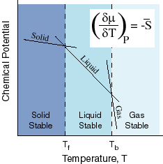Here we see the effects of temperature on the chemical potential. The slope of the chemical potential vs. Temperature line is the negative of the entropy. Thus, gases, which have large entropies, will have the steepest slopes and solids, which have the least entropies, will have the smallest slopes. Because they have different slopes, the lines cross. At the crossing points, one phase becomes more stable than another. We can see that at high temperature, the Gas has the lowest chemical potential, but at low temperature, the solid is lowest. In between, the liquid is lowest.

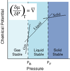
  The effect of pressure is sort of opposite that of temperature. Here the slope of the dependence of chemical potential on pressure is the molar volume. The molar volume of solids is low, but that of gases is high. Again the slope is greatest for the gas and least for the solid and thus the various lines cross. Where they cross, the phase changes. At low pressures, gases are favored. At high pressures, solids are favored.

 It is worth going through a short aside here. One can ask what the functional form of the G_m or the chemical potential is on pressure and temperature. Obviously, if the molar volume and molar entropy are constant, then changing the pressure at constant temperature or the other way around gives a linear plot (like the ones shown above). For example:

dG_m = V_mdP

when integrated for a constant V_m gives:

DG_m = V_mDP

Which we can see is a linear equation. This makes sense for solids and liquids which do not compress much (V_m is pretty constant with pressure), but obviously not for a gas. In that case, we can use the idea gas law for V_m remembering that this is for one mole so n = 1:

V_m = RT/P

dG_m = RT dP/P

Integrating

DG = RT ln(P_f/P_i)

The resemblance of this equation to the familiar

DG = RT ln(K_eq)

Is not a coincidence, but more on this at a later time. 

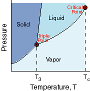This is a phase diagram. It takes the information from the last two diagrams and combines it showing where the phase boundaries are between the solid, liquid and gas phases. Notice that there is a place on the diagram where all three phases coexist. This is a special point called the triple point. Finally, there is something called the critical temperature above which there is no difference between liquids and gases (they have the same density at higher temperatures).

 I am not going to worry much about the derivation of phase boundries.

Now let's consider several topics by way of tutorials:

• Phase changes in a closed system with no atmosphere present.
• Phase changes in a closed system with atmospheric gases present.
• Phase changes in an open system.
• What causes the phase of a substance to change?

Below I describe something called the phase rule. It is useful for certain types of things, but the book does not describe it. I put it in for completeness, but will not test you on it:

In this we focus one equation: F = C - P + 2. This is the Gibbs phase rule. It applies to phases of a system which are in equilibrium with one another. Now all we have to do is to figure out what F, C, and P are.

P is the number of phases present (solid, liquid, gas). Note that there can be more than one phase of a particular type in multicomponent systems (such as oil and water which form two liquid phases).

C is the number of components present. This definition is kind of strange. The number of components in a system is the minimum number of independent species necessary to define the composition of all phases present in the system. The important word here is independent. If I have a chemical reaction, A à B +C, and if I know that I added a certain amount of A and formed a certain amount of B, then by stochiometry, I know the amount of C as well. C is not independent of A and B, so there are only two components. However, if I added an arbitrary amount of both A and B to begin with, then C would not be defined (because we messed up the stochiometry between A, B and C by adding extra B). In this case there would be three components. If there are no reactions, then the number of components is just equal to the number of chemical species present.

F is the number of degrees of freedom or variance in the system. This is the number of intensive variables like temperature, pressure or composition that can be changed independently without changing the number of phases. For example, if we have water at 25 C, we can change both the temperature and the pressure independently without changing the number of phases (which is one). Thus, there are 2 degrees of freedom. This is not true with an ice/water mixture. If we want to change the temperature and still maintain two phases, we will also have to change the pressure. Thus, there is only one degree of freedom. If we have a mixture of two miscible liquids (two liquids that freely mix) we have 3 degrees of freedom: the temperature the pressure and the composition of the mixture (mole fractions of the two components).

So the Gibbs phase rule allows us to predict how many degrees of freedom we have for a certain number of phases and a certain number of components. For the three cases above (water, ice/water and two miscible liquids) we see that it works. Water at 25 C has one phase and one component, so F = 2. Ice/water has 2 phases and one component, so F = 1. The two miscible liquids have 1 phase and 2 components, so F = 3. You should try and run through different examples for yourself and see if the equation makes sense.

It turns out that this is not an easy equation to derive precisely, but the concept is straightforward. Gibbs energy is a function of temperature and pressure, as we have discussed before. It can have only one value for any given temperature and pressure. At a phase boundary, the Gibbs energies of all phases present are equal. Now if I tell you that

G_liquid(T, P) = G_solid(T,P) you would realize that as long as this condition holds (as long as there is both ice and liquid water at equilibrium in your container), the system is constrained – if I change P, I must change T accordingly. There is one equation (one constraint) and two variables (P and T). The system is not uniquely determined, but there is a relationship that must exist between P and T. In other words, T becomes a simple valued function of P (or the converse). For any value of T there is a single corresponding value of P.

OK, but what happens if we have three phases in equilibrium (this happens at the triple point of water, for example). Now we can say that G_liquid(T, P) = G_solid(T,P) and G_liquid(T, P) = G_gas(T,P). There is one more constraint. We now have two equations constraining a system with two variables. Two equations, two variables, now the solution is unique. There can only be one value of T and P which will satisfy these equations.

F = C-P+2 is just a formal way of counting the number of degrees of freedom (related to the number of constraints (equations) and the number of variables which is always 2 – the reason a 2 appears in the equation). For a one component system:

The number of constraints (equations) = P-1.

This is because the number equilibrium relationships is always one less than the number of phases (for ice and water, there are two phases but only one relationship – that the gibbs energy of the two phases must be equal when they are both present).

The number of degrees of freedom = number of variables - the number of constraints = 2 – (P-1)

Or

F = 2 – P + 1

Which is exactly the equation above for one component (C=1). The fact that F cannot be less than zero means that for a single component system, you can only have 3 phases in equilibrium at any given time. Never any more. The point where all three are in equilibrium is called the triplet point.

Back to the main topics…

As for understanding the details of phase diagrams, I only want you to worry about the phase diagram for water below 2 atm in any detail. Water is weird stuff as described above, the phase boundry between liquid and solid angles backward with a negative slope in this pressure region. This is because ice is less dense than liquid water. These properties are critical for its role in living things, so you should be aware of them.

We now go from the behavior of a simple single substance to mixtures of substances. In general, these will still be non-reacting substances and we will be dealing mostly with the energetics of the mixing process itself and to a lesser extent with the types of nonideal interactions which can take place between different substances. We will also start to learn how to deal with liquid solutions, which will greatly increase our arsenal of systems that we know how to deal with.

First we must define the concept of mixtures. There are really two kinds of mixtures we will consider. One is a mixture of gases. This is usually discussed in terms of partial pressures as we have considered before. However, most of this chapter is devoted to the study of solutions and solutes. For example, in a solution of sugar dissolved in water, the sugar is the solute and the water is the solvent. Together they make up a solution.

We can talk about how much sugar is dissolved in the water in several ways. Most of the time, chemists (particularly biochemists) talk in terms of molarity – the number of moles solute per liter solvent. However, volumes of things are a bit misleading at times, because the ratio between the volume and the number of moles in not always constant. Many liquids expand with temperature or contract upon interaction with solutes. Thus it is generally more accurate to speak of molality – moles solute per kg solvent. The mass of the solvent does not change due to temperature or pressure or interaction with other molecules. The other way to talk about concentration is in terms of mole fraction – moles solute per total moles (solute plus solvent). Again this is independent of temperature and pressure. We will use these ideas in the description of mixtures below.

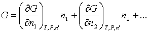
In order to talk about mixtures, we must define some way of specifying the values of thermodynamic parameters for components of a mixture. Such a description is provided by the concept of a partial molar quantity (think back to partial pressures – same idea). The formalism I will use is a bit more advanced than the book does (the book kind of jumps over this), and I am not going to require that you know the formalism below, I just present it as a way of learning the concept. If there is some parameter, X, that we wish to describe in terms of its partial value for each component of a solution then the value of X should just be the sum of the values of each of the contributions from the components. Of course, how much a particular component contributes to X will depend on how much of it is present. Thus we write:

This just says that any change in X will be given by how much the amounts of components 1, 2, 3… are changed (dn_i) and by the coefficient that tells us what the amount of X changes per mole of substance 1, 2, 3…, . These partial derivatives, by the way, are taken at constant T and P. These coefficients are called partial molar quantities. For small changes we can often integrate this expression and obtain:

The book, once again, avoids the partial derivatives. I think that once you get used to the idea of the partial derivative, their use is not only more correct, but easier to understand. In any case, you do not have to be able to perform derivations using the above formalism, but I want you to understand the concept of a partial molar quantity.

Lets consider an example. One common partial molar quantity is the partial molar volume. The partial molar volume of component i is just given by 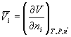. Thus it is the amount that the volume would change if we changed the number of moles of substance i on a per mole basis. The simplest case is a mixture of ideal gases, call them A and B. Note that in this case we hold T and P constant as well as the amounts of all other substances in the mixture (n'). We know that ideal gases do not interact and that their volumes depend only on how much is present at constant T and P: . Thus 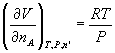. So it turns out that the partial molar volume of any component in a mixture of ideal gases is RT/P. It is not always that simple, but more on that later.

A more complicated example is a mixture of water and ethanol. These two substances form what is called an aziotrope at somewhere around 5% ethanol. At this point, the molar volume of ethanol is actually lower than the molar volume at any other point on the curve. This is because at this concentration, the interaction between ethanol and water is the strongest and ethanol fits appropriately into the hydrogen bonding structure of water.

OK, now we come to the really important partial molar quantity -- the partial molar Gibbs free energy. Just as for volume, we can write:

But we give a special name to the coefficients in this case, chemical potentials:

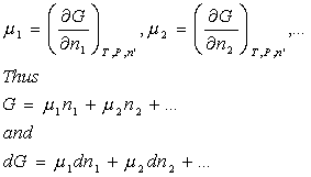
At constant temperature and pressure. In fact, we can just add these new terms to our previous expression for dG:

which reduces to the equation just above this if the temperature and pressure are constant.

An aside…

In principle, we could have written dG from the following equation differently

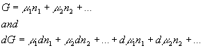
Yet from the arguments made above, we can see that this equation must be the same as the previous equation for dG:

Thefore

This is an important equation called the Gibbs-Duhem equation. What it says is that any change in the chemical potential of one component of a closed system must be balanced by another. This turns out to be a rather important fact. Don't worry about this particular equation (which we will not use much). Just realize that the values of individual chemical potentials in solution are intimately dependent on one another. The equations that we will need are the ones derived previously.

Back to the lecture… OK, but once again we are talking about things that look like absolute values. When I write:

G = n_Am_A + n_Bm_B + n_Cm_C

It sounds like absolute Gibbs energies or absolute chemical potentials. How does one deal with this? The answer is (again) that we use a reference state. We call the chemical potential of A in its standard state m_A⁰. Then starting with this (which is just some number), we can use what we know about how the molar Gibbs energy depends on temperature and pressure to calculate the chemical potential (which is really the molar Gibbs energy) at any temperature and pressure. Let’s do this for pressure. Remember that

dG_m = V_mdP (at constant T)

and for an ideal gas, we found that the change in G_m with P is

DG_m = RTln(P_f/P_i)

but the change in the molar Gibbs energy is just the same thing as the change in the chemical potential so,

Dm = RTln(P_f/P_i)

We can now rewrite our expression for G_i in terms of a reference state and a change from that state to the desired T, P, n:

G = G⁰ + DG = n(m⁰ + Dm) = nm⁰ + nRTln(P_f/P_i)

But in this expression P_i is the P of the reference state (we always do things relative to the reference state) and P_f is just the actual pressure P that we are dealing with. So we can write:

G = G⁰ + DG = n(m⁰ + Dm) = nm⁰ + nRTln(P/P⁰)

Now for a gas the reference state is defined at 1 bar. Now if you express your pressure in bars (1 bar = 10⁵ Pa which is very close to 1 atm), people often just leave it off completely (dividing by 1 is not very useful) and this gives:

G = G⁰ + DG = n(m⁰ + Dm) = nm⁰ + nRTln(P)

For a molar Gibbs energy (the usual way things are reported)”

G_m = G⁰ + DG = m⁰ + Dm = m⁰ + RTln(P)

Or just for the chemical potential of a particular species in the mixture:

m_i = m_i⁰ + RTln(P_i)

Where

G_m = m₁ + m₂ + m₃ + ...

You have to remember that this is sloppy notation and that the P in this equation is unitless because it really stands for P/P⁰. But, this is how chemists write out the equations for simplicity. We will find that we do exactly the same thing with concentrations. P has to be unitless, because it makes no sense to take a natural log of a Pascal.

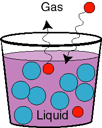
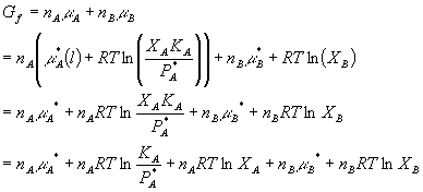
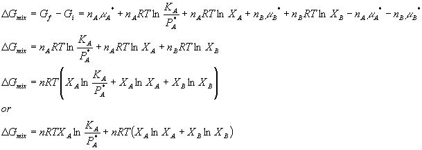
Ok, enough talk. What happens, then, to the Gibbs free energy if we take two pure ideal gases and mix them together? Consider gas A and gas B, both in separate containers at pressure P. Before we mix them, we can say that their initial Gibbs free energy total is just the sum of the individual Gibbs free energies:

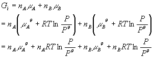
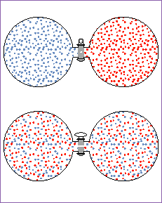Now lets mix them. As you can see in the diagram, both A and B now occupy the total volume of the system. Thus, the partial pressures of each are decreased. Therefore we have:

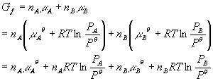
where P_A + P_B = P. You can see that the ratio term in the logs both got smaller, thus the entire value of the equation got smaller. This means that G_f < G_I which is what is expected for a spontaneous process. Just how big is the free energy change of mixing? Lets calculate DG:

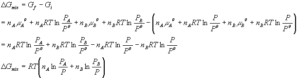
Sometimes it is convenient to write this in terms of mole fractions:

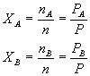
Which leads to:

These very simple ideas are extremely important. They tell us that simply by allowing different substances to mix together, the free energy of the system will drop (assuming that no negative interactions exist between the molecules -- we will explore that later). Remember the above results as presented are only exact for ideal gases.

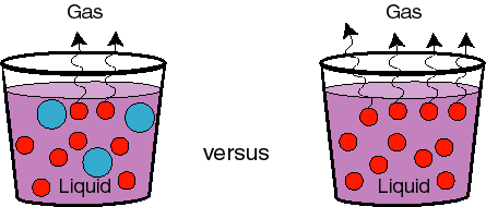
An obvious question at this point is, what happens if we mix two flasks with the same type of gas together at the same initial pressure? As you can see from the equations above, if the final mole fraction of the gas is 1.0, then the equation goes to zero. But why does it matter what the identity of the ideal gas is? This is interesting. It has to do with the fact that the driving force for mixing is actually the entropy change of the system upon mixing (see below). Mixing two buckets of balls together that are indistinguishable (have all properties in common) does not change the amount of disorder. But if you simply paint one bucket of balls red and the other green and then mix them, they become less ordered (the red balls are all mixed up with the green ones). It is probably not obvious to you why this changes the free energy. Lets try another example and perhaps it will make sense. In the picture here we have two different sized balls.

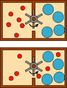The little ones can pass through the paddle and the big ones cannot. Because of this, the system can do work in exchange for mixing. However, if both sides had identical types of balls, it could not do work -- no change in Gibbs free energy. Anytime particles can be physically distinguished, there is the possibility of using those differences as big and little where used in this example. However, the mixing of indistinguishable particles cannot be coupled to performing work under any conditions.

We can also calculate the entropy and enthalpy of mixing for an ideal gas. Let's start with entropy. Remember what we are doing is to let all the A molecules occupy more space and all the B molecules occupy more space at constant pressure. Thus we have:

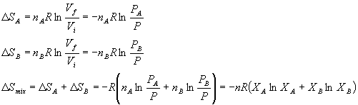
This looks awfully familiar. If we multiplied it by -T, we would get the Gibbs free energy. Thus for mixing of a two ideal gases:

The enthalpy being zero can be seen simply by comparison of the equation above it to

DG = DH - TDS

Finally, if you want to know what happens with the gases a start at different initial pressures, you just have to consider the value of the pressures of the two gases relative to one another.

Question you should now be able to answer: at what ratio of amounts of two ideal gases is the Gibbs free energy of mixing going to be the most negative (sounds like a good test problem to me)?

Ideal solutions

Our next job is to consider systems other than mixtures of ideal gases. The first one we will look at is ideal mixtures of liquids. Basically, an ideal solution or mixture of liquids is one where the vapor pressure of the liquid A is changed in proportion to its mole fraction when liquid A is mixed with liquid B. This will be true if the interactions between A and B molecules in the liquid is essentially the same as the interactions between A and A molecules and between B and B molecules.

Vapor pressure is the pressure due to A that would be generated if the gas molecules and the liquid molecules were allowed to come to equilibrium in a closed system. In fact, this is the key point, equilibrium. At equilibrium, the chemical potentials of the two phases of A (liquid and gas) are equal.

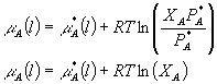
First, lets consider this for a pure liquid, A (we will use an * to denote a pure substance):

So at equilibrium, we have a simple way of getting the chemical potential for A in a liquid state. Now, if we mix two liquids together, the vapors will also mix in equilibrium above the liquid and the chemical potential of the vapor of A will depend on the partial pressure of A, just as before when we mixed ideal gases. We then have:

Next I am going to consider the difference in going from a pure liquid A to a mixture by subtracting the last two equations:

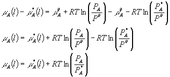
Notice something important -- we have done away with the standard chemical potential of the gas and have in its place as a standard state the chemical potential of the pure liquid A. Notice also something perhaps even more important. We have related the behavior of an ideal gas above the solution to the behavior of the solution. Suddenly we have a handle on solutions in terms of ideal gases.

Now, if the solution or mixture of liquids is ideal (which basically means that the interactions between like components of the solution are always the same as the interactions between different components) then the vapor pressure of A above the liquid will just be proportional to the molar fraction of A in the liquid. This is an important point and is called Raoult's Law:

Remember that here P_A* is the vapor pressure of A above a pure liquid A. In order to understand this at a molecular level, let's take a look at a tutorial.

Using this equation now, we can substitute:

See what we have now done -- all of the variables that depended on the vapor are gone and we are left only with parameters that are defined in the liquid phase. Also, since we have everything defined in terms of the liquid, we no longer need to worry about whether we are in equilibrium with the gas phase or not, since the properties shown are independent of the state of the vapor. This is a general expression for the chemical potential of some component A in an ideal solution of liquids.

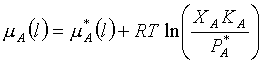
Ok, so the world is not an ideal place. The interactions between like components of the solution are not always the same as the interactions between different components, and Raoult's law does not work very well. In fact, there are relatively few situations for which Raoult's law is really very good. What do we do about that? We normally think of solutes as being at much lower concentration than solvents. Therefore the solute is always surrounded by solvent molecules. So it likely has a rather different interaction with the solvent than it does with itself, but at least since it is always surrounded by solvent, the interactions are always the same for essentially all of the molecules almost all of the time. This means we can think of the solute as having a characteristic dependent on the solute that surrounds it. As always, reality calls for a good fudge factor. We throw an extra empirical factor into Raoult's law and call it Henry's law. This fudge factor takes care of the fact that the solute surrounded by the solvent has different characteristics than the solute surrounded by itself (as was the case for pure systems).

Here K_A is the effective vapor pressure of component A when it is surrounded entirely by component B. Our chemical potential would now be:

We are still OK, because everything is still in terms of properties of the liquid (including the vapor pressure of the pure liquid). Note that Henry's law works well in general for very dilute solutions. Why? Because when A is in very low concentrations, it is surrounded almost entirely by B. Thus, it's enviroment is homogeneous -- it acts rather like a simple pure material again, even though it is in a mixture.

So, we use Henry's law to describe dilute solutions of liquids or (as explained below) solutes. These kind of dilute solutions are called ideal-dilute solutions.

At this point calculating the Gibbs free energy of mixing for ideal liquid solutions is a no-brainer. Remember for ideal gases that the chemical potential was given by:

and the Gibbs free energy of mixing was

where the mole fractions are mole fractions in the gas phase.

Well for the liquid, we have

where the mole fraction is now in the liquid phase,

and it should not surprise you to learn that the Gibbs free energy of mixing is just

In other words, the Gibbs free energy of mixing two ideal gases is the same as the Gibbs free energy for forming an ideal solution of two liquids. For more components, you just add more terms. The entropy and enthalpy of mixing are also the same as with ideal gases.

Remember, these equations only apply to ideal solutions! In real situations, the enthalpy, in particular, is usually not zero.

Let's just see what effects a mildly nonideal case would have on these. We can see that for ideal dilute solutions (Henry's law) instead of just X_A in the logarithm, we would have something proportional to X_A. As we saw before:

so for two components, we first consider them separately:

Now for a ideal dilute mixture where there is just a wee bit of A mixed in with a lot of B:

Now subtract the initial from the final Gibbs free energy:

How this extra term partitions itself between enthalpy and entropy depends on the details of the liquid interactions and structure. However, usually the bulk of the extra term ends up making the enthalpy of mixing nonzero.

Henry's law was one way of dealing with nonidealities, but really only works for very dilute solutions. We can more generally do the same thing by putting a fudge factor in front of the mole fraction in our chemical potential equation. This results in effective mole fractions or effective concentrations (see below). For liquids we give these the symbol 'a' and call them activities. Thus, we can write:

where the activity is just whatever it has to be in order to make the equation work. We can then write in terms of the activity coefficient, g,

which can be plugged in to give:

We get our ideal equation with some extra additive term that contains nasty realities in it. This term we consider to be empirical (although we will attempt to calculate it later for ions) and we write it down in a book somewhere. If you work back through the equations that we used to derive our chemical potential for a liquid mixture, you will find that we can also express the activity as:

where the top term is the actual vapor pressure of A when mixed with something else and the bottom term is the vapor pressure of pure A. This makes the activity coefficient simple to measure experimentally for solvents.

For ideal dilute solutions, remember we had (we will now call the solute B and the solvent A, for clarity):

or

people often lump the first two terms together and get:

m_B(l) = m_B⁰(l) + RTln (X_B)

We can now consider the effects of activity on the dilute solutions by writing:

m_B(l) = m_B⁰(l) + RTln (a_B)

Note that the activity in this case approaches the mole fraction as the concentration of the solute approaches zero (the Henry's law dilute-ideal condition). Thus the first term contains all the information about the system at some reference state (for this we will use a standard state, see below) and the activity corrects for the effects of the non-reference state.

Most of the time, we would rather deal with either molarity or molality than mole fraction. Molarity is moles per liter of solution. Molality is moles per kg of solvent. For precise work, we deal with molality, since volume depends on temperature (but mass does not). We can put the equation above in terms of activities based on molality. If you pick a standard state (usually 1 mole per kg solvent) and you consider the ratio m_B/m⁰ , where m_B is the molality of B and m⁰ is the standard molality, then we can rewrite our ideal chemical potential for the solute A as:

where now our new m_B⁰ is just the chemical potential of B in the standard state (usually 1 molal). We can then define an activity for this as well:

giving:

One of the important things in this chapter has been the definition of standard states. Remember that the standard state of a gas was 1 bar, the standard state of a solvent was the pure solvent and the standard state of a solute is 1 molal (1 mole solute per kg solvent). While these definitions are arbitrary, they affect everything we do from here on.

Colligative Properties

Ok, let's go back to simple, ideal mixtures of liquids for awhile and discuss various observable effects that change upon mixing liquids. Since we are considering the effects of changing the numbers of different molecules in solution, but not interactions (ideal solutions), these effects are effects that depend strictly on numbers of molecules and are thus called colligative properties (properties of a collection of molecules). For everything we talk about below, we will assume that we have some solvent A with a little bit of some solute B in it. We will further assume that B is nonvolital (does not contribute to the vapor pressure above the liquid) and does not incorporate itself into any solid which is formed upon freezing.

The first and most obvious of these is boiling point. The boiling point of a liquid is when the vapor pressure of the liquid is equal to the vapor pressure of the surrounding atmosphere. If we add something to the liquid which decreases its mole fraction below one, we have from Raoult's law that P_A = X_AP_A*. Thus, the vapor pressure of A in the mixture will be lower at any particular temperature than pure A. Thus the temperature required to achieve the point where the vapor pressure of the mixture is equal to that of the atmosphere will be higher in the presence of some solute B:

Another way to think about this, which is more general, is in terms of chemical potentials. The phase transition (boiling) will occur when the chemical potentials of the liquid and vapor phases are equal. But if we add something to the system, as we have seen before, the chemical potential of the liquid drops. Since the chemical potential of the ideal mixture is:

when X_A is less than 1.0, the chemical potential of the liquid drops and thus T will have to be greater before it reaches the point where the chemical potential of the liquid solution is greater than the chemical potential of the pure vapor (at which point the liquid boils). Note that the chemical potential of the vapor is not directly affected by addition of B since B is nonvolital. You can manipulate this formula to determine the change in the boiling point as a function of the amount of solute added. The result is

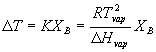
in the book, the constant terms are simplified to:

DT = K_Bm_B

where K_B is called the overall constant term in the equation and is called the ebulliscopic constant and m_B is the molality (rather than the mole fraction given above – as discussed before, these are interconvertable by converting moles of solvent to kg of solvent). Actually, the book uses the letter ‘b’ for molality. Much of the rest of the world uses ‘m’, so I will use the latter in the notes just to get you used to both conventions.

Deriving this equation takes a little work and I will not do it here (your book just states this formula without explanation). Basically, you look at what happens when you equate the chemical potential of the liquid and the gas phase, you realize that the difference between them is the gibbs energy of vaporization, you compare this to the situation for a pure solvent, you split the Gibbs energy change into enthalpy and entropy and realize that the entropy term cancels when you compare to the pure solvent. Finally you make a few approximations based on log functions. You don’t need to be able to do this, but I do want you to be able to use the above equation.

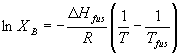
An almost identical argument can be made for the freezing point. Again, our solute only exists in the liquid phase and so it lowers the chemical potential for the liquid by not for the solid. The liquid in the presence of the solute is stabilized relative to either the gas or the solid phases. Thus it is harder to go to the gas (higher boiling temperature, see above) and harder to go from liquid to solid (lower freezing temperature). The equation describing the decrease in the temperature of fusion (the freezing or melting temperature) upon addition of solute is essentially identical to the one for boiling point elevation above:

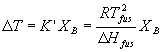
Again the book lumps together all the constants and converts mole fraction to molality giving:

DT = K_f m_B

Note, however, that the book has chosen to define DT differently in the two cases. This is very confusing (I do not know why they do this, but we are stuck with it). You simply have to remember that the change in temperature for boiling is an increase while that for freezing is a decrease. Let's consider an example of freezing point depression in a tutorial.

The next property is maximum solubility (this is not actually a colligative property, and the book does not actually cover this, but it fits in well here from the point of view of technique). Many times our solutes are not other liquids, but small amounts of some solid. If we add a great deal of a solid to a solvent and let them come to equilibrium, the chemical potentials of the solute in the solid and liquid should be the same. Let's call the solvent A and the solute B:

Now X_B is always less than one, so by making the mole fraction of the solute in the solvent low, we decrease the right side of the equation. If something is a solid at room temperature, that means that the chemical potential of its solid form is less than that of the liquid form. Effectively, however, in the presents of some solvent, we are lowering the chemical potential of the liquid form of the solute (the right side of the equation). The amount of B that can dissolve just depends on the mole fraction that makes the chemical potentials of the liquid and solid balance. Again the actual derivation is involved, but in the end we can express the mole fraction of solute present at saturation as:

Don't get too excited about this equation. It is darn near useless is reality because it does not take any solute/solvent interactions into account. However, it allows you to make rough guesses about how the solubility will depend on temperature for small temperature changes, and, more importantly, it is another conceptually good example of balancing chemical potentials. We won't use this one very much (the book does not use it at all), so don’t expect to need it on an exam. Just understand the logic of why the maximum solubility will depend on the things like the enthalpy of fusion and the temperature based on the arguments given above.

The final colligative property is Osmosis (this is in the book and you will need this equation). This is probably the most obvious example of a colligative property and it appears in many applications. Also, the equations tend to work pretty well over limited ranges of concentrations and temperatures, so the equation is useful. The picture below tells the story:

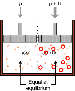
We have a liquid partitioned in two volumes. The two volumes are separated by a membrane that will let the solvent through, but not the solute (could have done it the other way around as well). To one side we add some solute, the other side is pure solvent. The side with the solute has a lower chemical potential. Thus, solvent from the pure solvent side will migrate through the membrane towards the side that has a lower chemical potential. The osmotic pressure is defined as the amount of pressure (in addition to atmospheric pressure) that one would have to apply to the side that has the solute in it in order to keep more solvent from going over to that side. Again, by balancing the chemical potentials, one can show that the pressure required is just:

where [B] is the molarity (number of moles per liter) of solute in the solvent. To derive this you have to go back to the issues of vapor pressure and Rauolt’s law and Henry’s law and change the pressures to allow the two sides to be in equilibrium.