The title of this page may seem backwards to you if you have not thought much about such things. You might think, why would I want to reduce my data and analyze my error? Don't I want to analyze my data and reduce my error? Well, reducing error is an experimental art -- once you have taken the data, the error is what it is and you can only determine its extent, not reduce it. As for reducing data, that is, in fact, what we generally do -- we reduce our data to a small number of physically significant values. For example, if I measure the pH of a solution 10 times and then average the measurement to get one value, I have reduced my data from ten numbers to one more significant number. If I take 20 absorbance values at 20 different concentrations of dye and then fit the results to a line, I am reducing 20 pairs of numbers to a single pair of numbers (a slope and an intercept). Thus, much of quantitative science really is a matter of reducing our data down to a small number of meaningful parameters and then analyzing the error in those parameters.

Distributions of errors

How do we go about this? Let's start with the simplest case -- averaging a group of numbers to get an average. First, we must make an important assumption. Note, this assumption is very often not true in the real world and must be considered carefully. We are going to assume that our errors are normally distributed about the real value. What does this mean and why would we do it? The normal or bell curve is a function of the form:

Here x is the value you measured, m is the average (mean) of the values you measure, and s is something that relates to how wide the distribution of values about the average is (we will see in a moment that it is the same as the standard deviation of the values). This curve is shaped like a bell with the maximum at the point where x = m and going down on either side. It is the probability density of finding a particular value of x in the experiment. To get a real probability we would have to integrate. For example, I could ask, what is the probability of finding experimentally that x = 2.10000 when the average value of x was 2.00000. Well the problem with asking that question is that the probability of finding the value 2.10000 is zero, because there are an infinite number of possible values for x. I need to ask, what is the probability of x being between 2.1 and 2.2 . To get this, I would integrate the equation above over the range of x from 2.1 to 2.2 and get a real probability. Thus, we essentially always deal with integrals of this equation. Unfortunately, there is no analytical solution to the indefinate integral of that equation, so we have to calculate it numerically or look it up in a table somewhere. But, hey, that's what computers are for.

Where did the normal distribution come from and why would you use it? Perhaps an example is better than a proof. If you were to take a coin and flip it 100 times and count the number of heads, (assuming a perfectly symmetric coin and such) you should find on average that there should be 50 heads. However, if you really did this many times, of course you would not always get 50 heads. Most of the time you would get something else. However, you would find that you are more likely to get 50 heads than 49 (or 51) heads and more likely to get 49 (or 51) heads than 48 (or 52) heads, etc. In fact, the distribution would drop off in both directions according to the equation above (approximately -- not perfectly-- because you are physically limited to getting a positive number of heads less than or equal to 100, while the equation covers minus to plus infinity, but this would be a very small effect). You can verify this by calculating the probabilities and comparing them to the shape of the curve above if you like. It works.

Note that there are many types of systematic errors in the world that do not follow a normal distribution. For example, if your pH meter is drifting during your series of measurements, this will give rise to a systematic error and cannot be analyzed by the kind of error analysis we are talking about here. The solution? Fix your pH meter.

Standard distribution

OK, so how do we characterize the width of the distribution of errors in a set of measurements? Let's look again at the normal distribution equation:

You can see from the equation that if s² is a small number, it will mean that when you change x, there will be a big change in the value of the function (the slope of the side of the bell curve becomes steep). If, on the other hand, s² is a large number, then a change in x does not have as large an effect on the value of the function. The bell curve has shallow slopes and is thus broader. Thus, s² is apparently directly related somehow to the width of the distribution. It turns out that s² is basically the average squared error (in other words the average of the value ). I would have to go through a pretty long statistical argument to prove this to you in general -- we would have to define some case like the coin flipping case (or something more general and continuous) and show that the statistics followed the above equation when s² was the average squared error in the system. I am not going to do this. However, from this argument, one might conclude that:

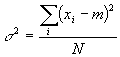
However, this is not quite true. Look what happens at small N (N is the total number of measurements taken). If N=1, for example, then there is only one value measured. Clearly under these conditions we can say nothing about the error in the measurement. Yet this equation says the error is zero! So, for the narrowest error distribution, just do the experiment once and never repeat it, right? Wrong. This makes no sense. The error after one experiment is undefined. This fact is reflected in the slightly modified version of the above equation that we all know and love as the variance or (after taking the square root of both sides) the standard deviation

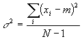
In this equation, the standard deviation is undefined for one measurement because for one measurement the top is zero (a single measurement value is its own average) and the bottom is zero. This, then, is what we typically report as the standard deviation (s) of a group of numbers.

The standard deviation is not the same as the error in the mean.

So far, we have talked only about distributions of individual errors, not the error associated the average of a bunch of numbers. In other words, when you take 10 pH readings and average them and determine a standard deviation, that is not the error in your determination of the average, it is the standard deviation of an individual measurement -- the amount you can expect individual measurements to vary from time to time. Note that the value of the standard deviation above does not decrease as N increases. This is because the sum of the squared error goes up just as fast as N. We will later discuss how to determine the error in the mean of a bunch of measurements.

Propagation of errors.

OK, so let's suppose that you have measured the pH of some solution and determined its standard deviation (by measuring it many times) and you have also used absorbance spectroscopy to determine the ratio of the concentrations of the acid and base forms of the molecules that are picking up or letting of protons in the solution, and you have standard deviations for both of these values:

R is the ratio of the concentrations of the base form to the acid form. This is the Henderson-Hasselbach equation with the errors of the values explicitly stated. So, you know all the values and their errors on the right hand side of the equation, but what is the error of the pK_A that you calculate? This is called propagation of error. You may have been told how to do it for simple cases before, but how do you do it in general?

It works like this. Let's say we have some function, f(x,y). We know the errors in x and y and we want to know the error in the value of the function. From past classes (I know you all had chm341), you know that a small change in the x and y values can be used to determine a small change in the f value:

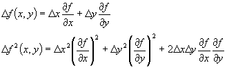
Now it turns out that as long as the errors in x and y (the changes in x and y) are not correlated (they are random relative to each other) the last term cancels out on the average. This is because it is positive part of the time and negative part of the time. The other two terms are always positive. Thus, if we consider our standard deviations to be the small changes in x and in y, then we can calculate the standard deviation in f as follows:

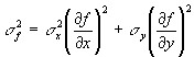
That is it then, the general formula for propagating errors. Let's try it on the H-H equation below.

So, f (the function) is the pK_A and the two variables are pH and R (instead of x and y). So,

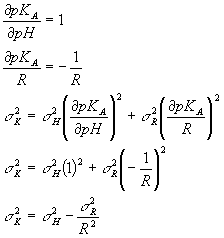
So now from the standard deviation of your pH data and your ratio data (R), you can calculate the standard deviation value you would get for the pK_A. Be careful. This is again the width of the distribution of pK_A values you would get if you measured a bunch of separate pH and R values, calculated a bunch of separate pK_A values and then looked at the standard deviation of those pK_A values.

Error of the mean value of a series of values.

Let's try that last problem again, but this time, let's say we wanted to know the error in the mean value of the pK_A. In other words, we are going to measure our pH and R values many times, average them, get more accurate pH and R values than any single measurement could give, and then calculate the pK_A and its error. How do we do this? Well, how do we calculate the error in an average of a bunch of numbers? The average is given by:

Remember the standard deviation of the x values is the amount of error we might expect for each individual reading due to our instrument uncertainty. Thus each of the x_i values has an error of s_x. How do we find out the error in the mean? The same way we found out the error in the pK_A, propagate the errors. The mean is a function of all the x_i values, but each of the x_i values has the same standard deviation (individual error).

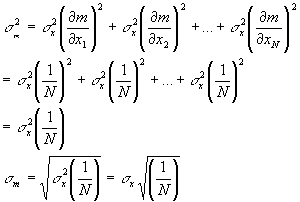
So the actual error in the average value of the numbers is just the standard deviation divided by the square root of 1/N. Unlike the standard deviation, this value decreases with increasing number of measurements. The more measurements you average, the smaller your error in the mean. The error in the mean decreases as the square root of one over the number of measurements. Thus, to decrease the error of your measured values by a factor of 2, you must average 4 measurements. To decrease the error of your averaged values by a factor of 10 you must do 100 measurements, etc. Now for the H-H equation we can use the error in the mean as the error in the averaged pH and R values and from this determine the error in the pK_A value that is calculated from the average pH and R values, just as we did for standard deviations (same formula, but use the error in the mean in place of the standard deviation both for pH and R).

You try it (these kinds of problems might be on the final)

The table below contains a set of pH and ratio (R) values to be used in the H-H equation to calculate the pK_A.

a) Calculate the average and standard deviation, and error in the mean of the pH and R.

b) Calculate the average, standard deviation and error in the mean of the pK_A using propagation of errors.

c) Calculate the average, standard deviation and error in the mean of the pK_A by calculating pK_A for each individual set of pH and R values and then performing an analysis of those numbers.

d) For the equation f(x,y) = x² + sin(y), propagate the errors in x and y and determine the resulting error in f.

ANSWERS

Linear regressions

There are many instances where instead of taking a series of numbers and simply averaging them, you take a series of pairs of numbers and you have some model for how they should relate to one another. The simplest example is a line. Let's say you have a set of dye concentrations and an absorbance value for each concentration. Beer's law says the two should be linearly related (A = ecl, as you recall). However, your spectrophotometer has some offset associated with it that you were unable to zero when you started your measurement, so everything has a constant added to it resulting in A = ec + B, where B is the baseline offset (we will assume that the pathlength, l, is 1 cm). You want to fit your data to a line (A as a function of c) which should have a slope of e and an intercept of your offset B. How do we determine the best e and B for the data you have taken?

Obviously, we want to pick values of e and B that give a line that comes as close as possible to all of the points. In other words, we would like the error between the values for A and the values for ec + B, for each concentration and absorbance, to be as close as possible. Thus, you might guess that we should look for a minimum in the following function:

In other words, find values of e and B such that the sum of all the errors between the measured absorbances and the absorbances calculated from the measured concentrations is as close to zero as possible. The problem is that since each of the errors can be positive or negative, there could be very big errors that cancel and still sum to zero. Thus, this is not the right criterion. We want all of the errors to add up in a positive way to give a total error. We could use an absolute value, but absolute values are not well behaved near zero (the derivatives blow up) and thus would be hard to work with. So, we will choose to use the square of the errors and add all those up.

This type of error calculations is called a chi squared error. Now, this is not so strange. It looks a lot like the way we dealt with errors in single numbers before. Remember we used the sum of (x_i - m)². Well m was the theoretical value (the average value) just as ec_i + B is the theoretical value (the line value) here. We need to find the correct values of e and B that minimize the chi squared error. We can do this like we minimize any function. Take derivatives and set them to zero. Before we do this, let's use a more general equation of a line and rewrite the chi squared error expression in terms of the more general linear equation:

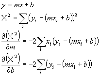
Now we just set each of the derivatives to zero to find the minimum:

N is the number of data pairs we have and is just the sum over i of 1. Now the important thing to realize here is that all those sums are just sums of numbers we measured (absorbances and concentrations). They are, themselves, just simple numbers from our data. In fact, to make it simple, lets just give those sums simple names and rewrite the equations:

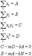
Now we just solve (2 equations and 2 variables, m and b):

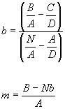
So all we have to do is to calculate each of the sums from our data (A, B, C and D) and then plug into the above equations to get the best possible slope and intercept of the line to fit the data.

Now this can be done for more than just lines. Any function will work. However, only certain functions (functions that are linear in the parameters of the fit) will yield sets of equations that can be solved analytically. But if we can't solve them analytically, we solve them numerically with a computer.

How do errors come into all of this? Well, we can calculate our errors in the various sums of the data and just propagate them into the slopes and intercepts in the usual way.

Often, however, the error in the dependent variable is much larger than the error in the independent variable. In other words if we are measuring y as a function of x, very often we have set x ahead of time and there is very little error, but the measurement of y is error prone. In this case, we can see that (y_i -(mx_i + b))² should have the same value as the error associated with measuring y_i (called s_i below). Thus, we often rewrite the equation for the chi squared error as:

This is called the reduced chi squared and has the useful property that if the line fits the data to within the noise of the measurement of y, then the reduced chi squared should have a value of about 1.0. If the value is larger than this, it means that a line is not an adequate description of the data to within the noise.

Try it out

The following is a set of concentrations and absorbance values.

a) Use the equations above to determine the best fit to a line (just this once, do it by hand without using the linear regression button on your calculator).

b) Assuming that the errors in the concentrations are plus or minus 10 mM and the errors in the absorbances are plus or minus 0.001, determine in the error in the extinction coefficient and the instrument offset that you have calculated. (Note, most automatic functions on calculators do not do the error calculation for you).