This page last updated on January 26, 2023, 5:45AM MST.
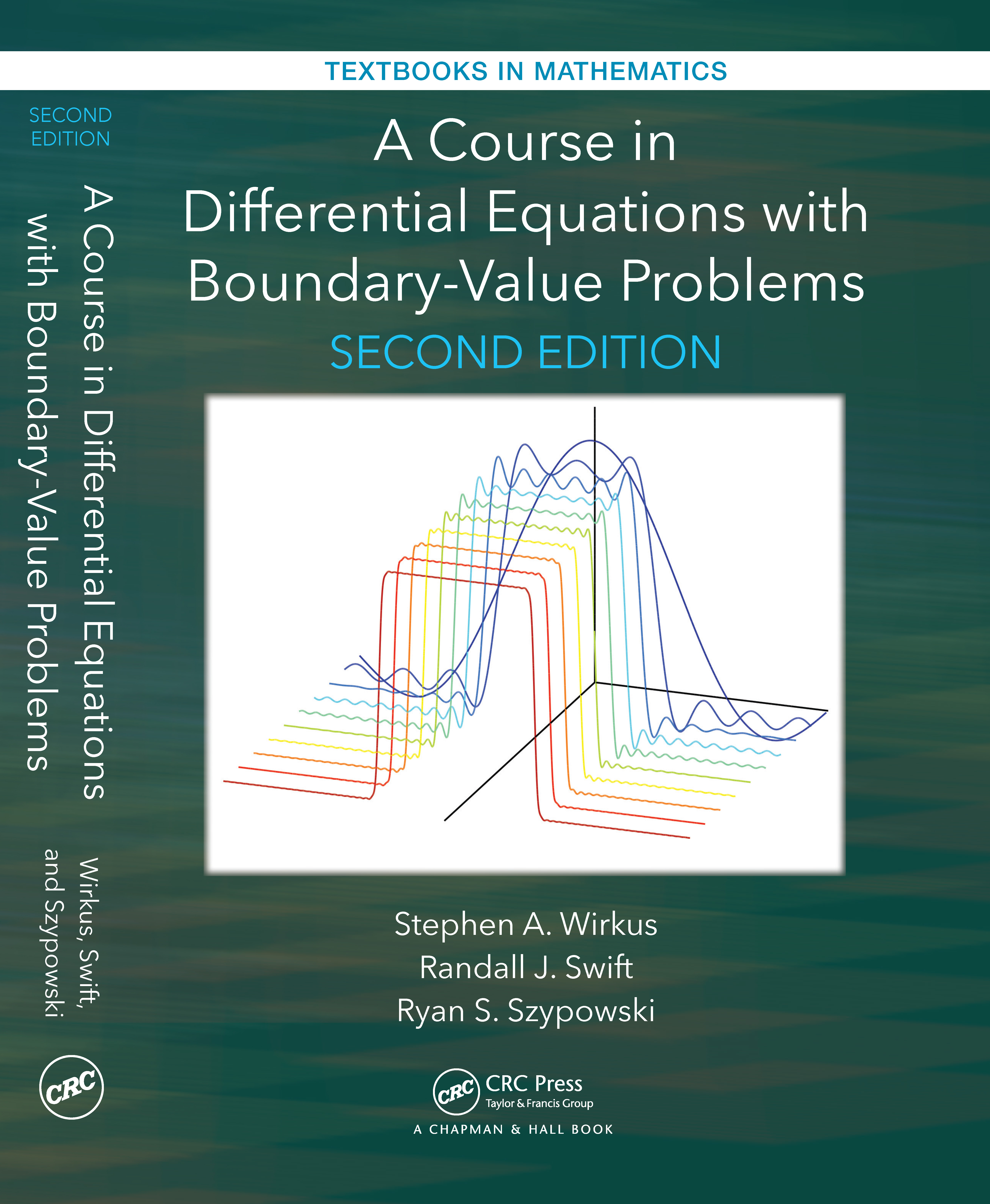
A Course in Differential Equations with Boundary-Value Problems, 2nd Edition

A Course in Differential Equations with Boundary-Value Problems, 2nd Edition
Find the book at
CRC Press or at
Amazon.
You can see reviews of the first edition (both professional and student) at
Amazon.com.
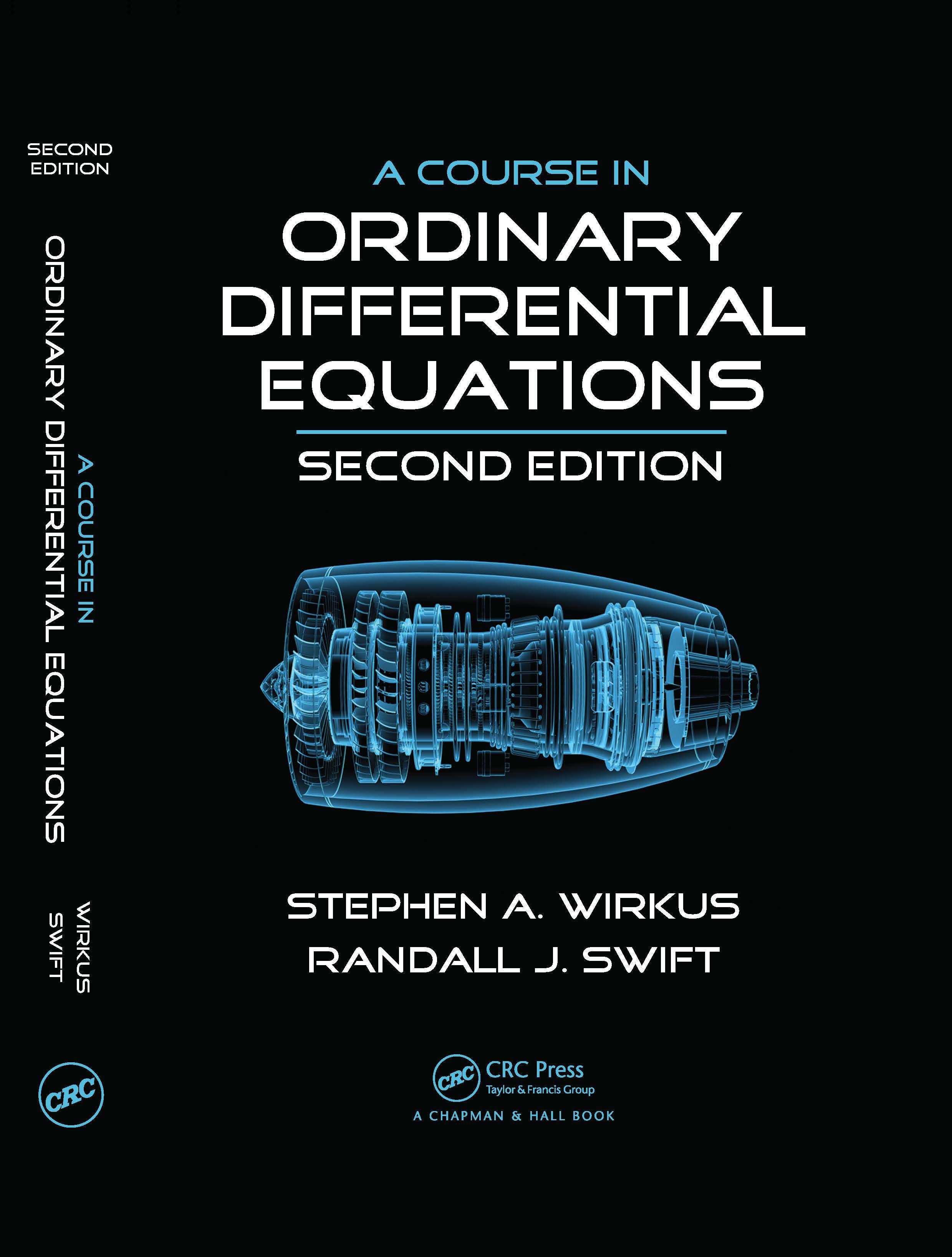
 The webpage for A Course in Ordinary Differential Equations, 2nd Edition by Wirkus and Swift can be found by clicking on the book to the left.
Additional information on A Course in Differential Equations with Boundary-Value Problems (book to the right) can be found by clicking on the topics below or scrolling down the page.
Summary
Table of Contents
Author Biographies
Features
New to the Second Edition
Computer Labs
Typos and Errata
A Course in Ordinary Differential Equations, Second Edition teaches students how to use analytical and numerical solution methods in typical engineering, physics, and mathematics applications. Lauded for its extensive computer code and student-friendly approach, the first edition of this popular textbook was the first on ordinary differential equations (ODEs) to include instructions on using MATLAB, Mathematica, and Maple. This second edition reflects the feedback of students and professors who used the first edition in the classroom.
(back to top)
Chapter 1: Traditional First-Order Differential Equations
1.1. Introduction to First-Order Equations
1.2. Separable Differential Equations
1.3. Linear Equations
1.4. Some Physical Models Arising as Separable Equations
1.5. Exact Equations
1.6. Special Integrating Factors and Substitution Methods
Chapter 2: Geometrical and Numerical Methods for First-Order Equations
2.1. Direction Fields---the Geometry of Differential Equations
2.2. Existence and Uniqueness for First-Order Equations
2.3. First-Order Autonomous Equations---Geometrical Insight
2.4. Modeling in Population Biology
2.5. Numerical Approximation: Euler and Runge-Kutta Methods
2.6. An Introduction to Autonomous Second-Order Equations
Chapter 3: Elements of Higher-Order Linear Equations
3.1. Introduction to Higher-Order Equations
3.2. Linear Independence and the Wronskian
3.3. Reduction of Order---the Case n = 2
3.4. Numerical Considerations for nth-Order Equations
3.5. Essential Topics from Complex Variables
3.6. Homogeneous Equations with Constant Coefficients
3.7. Mechanical and Electrical Vibrations
Chapter 4: Techniques of Nonhomogeneous Higher-Order Linear Equations
4.1. Nonhomogeneous Equations
4.2. Method of Undetermined Coefficients via Superposition
4.3. Method of Undetermined Coefficients via Annihilation
4.4. Exponential Response and Complex Replacement
4.5. Variation of Parameters
4.6. Cauchy-Euler (Equidimensional) Equation
4.7. Forced Vibrations
Chapter 5: Fundamentals of Systems of Differential Equations
5.1. Useful Terminology
5.2. Gaussian Elimination
5.3. Vector Spaces and Subspaces
5.4. Eigenvalues and Eigenvectors
5.5. A General Method, Part I: Solving Systems with Real & Distinct or Complex Eigenvalues
5.6. A General Method, Part II: Solving Systems with Repeated Real Eigenvalues
5.7. Matrix Exponentials
5.8. Solving Linear Nonhomogeneous Systems of Equations
Chapter 6: Geometrical Approaches and Applications of Systems of First-Order Equations
6.1. An Introduction to the Phase Plane
6.2. Nonlinear Equations and Phase Plane Analysis
6.3. Bifurcations
6.4. Epidemiological Models
6.5. Models in Ecology
Chapter 7: Laplace Transforms
7.1. Introduction
7.2. Fundamentals of the Laplace Transform
7.3. The Inverse Laplace Transform
7.4. Translated Functions, Delta Function, and Periodic Functions
7.5. The s-Domain and Poles
7.6. Solving Linear Systems using Laplace Transforms
7.7. The Convolution
Chapter 8: Series Methods
8.1. Power Series Representations of Functions
8.2. The Power Series Method
8.3. Ordinary and Singular Points
8.4. The Method of Frobenius
8.5. Bessel Functions
Chapter 9: Boundary-Value Problems and Fourier Series
9.1. Two-Point Boundary-Value Problems
9.2. Orthogonal Functions and Fourier Series
9.3. Even, Odd, and Discontinuous Functions
9.4. Simple Eigenvalue-Eigenfunction Problems
9.5. Sturm-Liouville Theory
9.6. Generalized Fourier Series
Chapter 10: Partial Differential Equations
10.1. Separable Linear Partial Differential Equations
10.2. Heat Equation
10.3. Wave Equation
10.4. Laplace Equation
10.5. Nonhomogeneous Boundary Conditions
10.6. Non-Cartesian Coordinate Systems
Appendix A: An Introduction to MATLAB, Maple, and Mathematica
A.1. MATLAB
A.2. Maple
A.3. Mathematica
Apprendix B: Selected Topics from Linear Algebra
B.1. A Primer on Matrix Algebra
B.2. Matrix Inverses, Cramer's Rule
B.3. Linear Transformations
B.4. Coordinates and Change of Basis
Answers to Odd Problems
References
Index
A Review, Computer Labs, and Projects appear at the end of each chapter.
(back to top)
Stephen A. Wirkus completed his Ph.D. at Cornell University under the direction of Richard Rand. He began guiding undergraduate research projects while in graduate school and came to Cal Poly Pomona in 2000 after being a Visiting Professor at Cornell for a year. He co-founded the Applied Mathematical Sciences Summer Institute (AMSSI),
an undergraduate research program jointly hosted by Loyola Marymount University, that ran from 2005 through 2007. He came to Arizona State University in 2007 as a tenured Associate Professor and won the 2013 Professor of the Year Award at ASU as well as the 2011 NSF AGEP Mentor of the Year award. He was a Visiting MLK Professor at the Massachusetts Institute of Technology in 2013-2014. He has guided over 80 undergraduate students in research and has served as Chair for 4 M.S. students, and 6 Ph.D. students. He has over 40 publications and technical reports with over 40 students and has received grants from the NSF and NSA for guiding undergraduate research. In 2022-2023, he served as a Program Director in the Division of Mathematical Sciences (DMS) at the National Science Foundation.
Randall J. Swift completed his Ph.D. at the University of California, Riverside under the direction of M. M. Rao. He began his career at Western Kentucky University and taught there for nearly a decade before moving to Cal Poly Pomona in 2001 as a tenured Associate Professor. He is active in research and teaching, having authored more than 80 journal articles, three research monographs and three textbooks in addition to serving as Chair for 25 M.S. students. Now a Professor, he received the 2011-12 Ralph W. Ames Distinguished Research Award from the College of Science at Cal Poly Pomona. The award honors Swift for his outstanding research in both pure and applied mathematics, and his contributions to the mathematics field as a speaker, journal editor, and principal investigator on numerous grants. He was also a Visiting Professor in 2007-2008 at The Australian National University in Canberra Australia as well as having taught at the Claremont Colleges.
Ryan S. Szypowski completed his Ph.D. at the University of California, San Diego under
the direction of Michael Holst. He was hired at Cal Poly Pomona in 2011 and became
a tenured Associate Professor in 2016. His main research is in the area of computational
methods for approximation of solutions to partial differential equations, but studies broad
problems from applied mathematics and science with his students and colleagues. He had
an active NSF research grant from 2012 to 2015 to study adaptive techniques in �nite element exterior calculus and has won numerous smaller grants to support his work with
students. In 2015, he won the Department of Mathematics and Statistics Excellence in
Teaching Award.
(back to top)
- Describes analytical and numerical methods for studying ODEs, BVPs, and PDEs
- Shows students how to effectively use MATLAB, Maple, and Mathematica in practice, assuming no prior knowledge of the software packages
- Covers essential linear algebra topics, such as eigenvectors, bases, and transformations, to improve students' understanding of differential equations
- Includes numerous problems of varying levels of difficulty for applied and pure math majors as well as for engineers and other nonmathematicians
- Offers answers to most of the odd problems in the back of the book
- Contains reviews and projects at the end of each chapter
- Solutions manual available upon qualifying course adoption
(back to top)
- Moves the computer codes to Computer Labs at the end of each chapter, which gives professors flexibility in using the technology
- Covers linear systems in their entirety before addressing applications to nonlinear systems
- Incorporates the latest versions of MATLAB, Maple, and Mathematica
- Includes new sections on complex variables, the exponential response formula for solving nonhomogeneous equations, forced vibrations, and nondimensionalization
- Highlights new applications and modeling in many fields
- Presents exercise sets that progress in difficulty
- Contains color graphs to help students better understand crucial concepts in DEs
- Provides updated and expanded projects in each chapter
- Suitable for a first undergraduate course, the book includes all the basics necessary to prepare students for their future studies in mathematics, engineering, and the sciences. It presents the syntax from MATLAB, Maple, and Mathematica to give students a better grasp of the theory and gain more insight into real-world problems. Along with covering traditional topics, the text describes a number of modern topics, such as direction fields, phase lines, the Runge-Kutta method, and epidemiological and ecological models. It also explains concepts from linear algebra so that students acquire a thorough understanding of differential equations.
(back to top)
Typos last updated on January 26, 2023, 5:45AM MST.
Note on electronic book vs hard copy: the electronic version appears to be numbered somewhat differently. I have not seen this to compare but, for example, p.661 in the electronic book is p.650 in the hard copy. Please keep this in mind as you go through typos. I will refer to sections for this reason.
Where convenient, missing or changed items are highlighted in the lines below.
p. 73 (problems in section 2.1): In Problem 24, point is (0,1).
p.117 (gray box, MATLAB, Example 3): In the RK4.m code given in the computer lab/gray MATLAB section at the end of chapter 2, the 8th and 9th lines should be corrected with the highlights below:
xout(i +1,:)=xnext;
yout(i +1,:)=ynext';
p.260 (gray box, MATLAB, Example 4): In Example 4 of Computer Lab 4, apostrophes were omitted in 7 lines. The corrections are with highlights below:
wn=sym('wn','real')
wn=sym('wn','positive')
F0=sym('F0','real')
F0=sym('F0','positive')
m=sym('m','real')
m=sym('m','positive')
t=sym(' t ','real')
p. 321 (Section 5.7, Example 3): Eq. (5.110). The top right entry should be (-1/3)*exp(3) + (1/3)*exp(-3)
p. 340 (gray box, MATLAB, Example 4): The matlab formula in the last line of this example is missing a parenthesis at the end; it is supposed to match the equation in the book in the line before (5.82) on p.313:
soln = c1*exp(E(1,1)*t)*V(:,2) + c2*exp(E(1,1)*t)*V(:,1) + c3*(t*exp(E(1,1)*t)*V(:,1)+exp(E(1,1)*t)*(equ v1))
p. 460 (Section 7.5, Example 7): The ODE in Example 7 should be (D2+3D+2)(D2+6D+10)(x) = E′′+4E
p. 460 (problems in section 7.5): Problem 10 should be x′′ + 4x' + 5x = E′ + 32E
p. 464 (problems in section 7.6): In Problem 9, the second equation should be "x'-3x+y'-3y=2" (i.e., remove the ' from -3y')
p.473 (gray box, MATLAB, Example 3): In Example 4 of Computer Lab 7, apostrophes were omitted in 7 lines (typo identical to above p. 260). The corrections are with highlights below:
wn=sym('wn','real')
wn=sym('wn','positive')
F0=sym('F0','real')
F0=sym('F0','positive')
m=sym('m','real')
m=sym('m','positive')
p. 645. (gray box, MATLAB, Example 1): In Example 1 of MATLAB code, 2nd line is missing a period on the rhs of the equation:
f = @(t) t.^2;"
Thank you for reporting the above typos and errata. We appreciate your support!!
Send additional ones to:
Stephen Wirkus (e-mail: swirkus "at" asu "dot" edu)

Website Stats

 The webpage for A Course in Ordinary Differential Equations, 2nd Edition by Wirkus and Swift can be found by clicking on the book to the left.