Chemical Dynamics

Chapters 6 and 7

Up until now we have considered thermodynamics which tells us whether a reaction is spontaneous or not and how much energy is involved in various different forms. Thus, in principle, we can state whether or not some particular process will happen, but we have no way of knowing how long that process will take or what path it will take to go from the initial to the final state. In order to understand this, we must study chemical dynamics.

Much of the field of chemistry is discussed in terms of systems that are static at the time of observation. We perform chemical reactions and consider the structure or chemical properties of the reactant and product. Yet the chemistry is in the reaction itself, and that is clearly a dynamic process. One can infer a great deal from the static properties of molecules, but much of our knowledge of reaction mechanism relies on the observation of the time dependence of chemical reactions.

What can one learn from reaction kinetics? Most of the time in studies of chemical kinetics, what one is doing is relating the time evolution of the population of some molecular species (the observable) to a model for the mechanism of the reaction taking place. Several types of information can come out of such a study. First, one can learn what the path of the chemical reaction is. This information typically comes from comparing the expected results from a series of possible kinetic pathways to the actual time dependence of the molecular population observed. Next, one can learn what the specific rates are for different reaction steps. This in turn provides information about what limits the rate (and often the yield) of chemical reactions. By varying conditions, such as temperature or solvent type, one can learn what type of energetic barriers must be overcome in order for a reaction to proceed.

A few applications of chemical kinetics. Kinetic analysis has been applied to many systems in order to learn more about the reaction mechanism. For example, let's say that you are converting one mixture of chemical species, A and B, to another mixture, C and D, by heating for a period of time and you want to learn something about the nature of the reaction. One simple question you can ask is, "what type of reaction limits the rate of the overall conversion?". By looking at the kinetics of the reaction as a function of reactant concentrations, one can determine if the rate limiting step is the formation of an interaction complex between the reactants, the resolution of this complex into the products, or a unimolecular conversion of one of the reactants or reaction intermediates to a different form before the reaction can take place.

One common application of kinetics in biochemistry is the study of enzyme kinetics. An enzyme is a catalyst, and the kinetics of enzymes is similar to the kinetics of other catalytic reactions. Questions that can be addressed by looking at the kinetics of an enzyme reaction are: how strong is the interaction between the reactants or products and the enzyme, are there other molecules which affect the rate of the reaction (but are not themselves used up) besides the enzyme, and are reaction rates limited by diffusion?

Another interesting application of standard kinetic theory is electron transfer reactions in a solid state (i.e. first order) system. This is often used to model electron transfer in either respiratory or photosynthetic systems in biochemistry. In this case, one typically looks at either the optical spectrum or the electron paramagnetic resonance spectrum as a function of time to identify reaction intermediates and to investigate the reaction mechanism.

In these chapters, we will consider the basis for multiorder and first order kinetics, with emphasis on the application of kinetic information in determining reaction mechanism. Then we will discuss in more detail what actually determines the individual rate constants of a reaction and explore some biochemical applications.

The rate of a chemical reaction. Much of the experimental aspect of chemical kinetics is concerned with the measurement of reaction rate. There are a couple of points worth making about this. First, the rate of a reaction is the change in the concentration or population of some reaction component with time.

This is not always as straightforward as it sounds. First, how you define the rate may well depend on which reactant or product you are interested in. For example in the reaction Aà B the rate of the reaction could either be expressed in terms of the change in [A] with time or the change in [B] with respect to time. The two rates are just negative of one another:

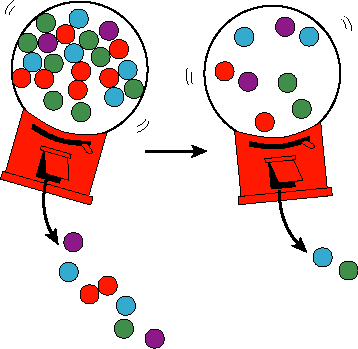
Second, rates are typically concentration, and therefore time, dependent. Thus, there is no single rate for a reaction. To simply say, reaction A is faster than reaction B has very little meaning without specifying all the concentrations of the components involved. For example, consider the rate at which marbles come out of a small hole in a container. If the container has many marbles in it, then many marbles happen to hit the hole and pop out in any given period of time. However, if the number of marbles is small, then the rate at which marble will come out is slower.

As chemists, we would like to be able to compare reaction kinetics quantitatively. Thus, we need to come up with some parameters related to the reaction kinetics which are concentration independent.

Rate constants. Consider the simple irreversible (i.e. no back reactions) reaction

The instantaneous rate of the reaction at any time, t, is just the derivative . Note that for simplicity I will sometimes refer to the time dependent concentration of a molecule as, for example, A(t), rather than using brackets, [A]. Now, what will this reaction rate depend on and what should the functional form be? What assumption is used to relate the rate of A's demise to its instantaneous concentration in a linear manner? The fundamental assumption is that individual molecules have no memory. In other words, all A molecules have the same probability of converting to B in a given period of time regardless of their history. More generally, we assume that any particular molecule of A is identical to any other not only at the present time but at any past or future time. If this is true, than the instantaneous probability that any particular molecule of A will change to B is time independent. This instantaneous probability, then, is a useful constant for comparing irreversible first order reactions.

Ok, but what is an instantaneous probability and how does it relate to a normal probability? Well, let's say you are star gazing out in the woods at night and you are looking for shooting stars (OK, meteorites, since this is a science class). You watch for 30 minutes and you see 33 meteorites. What is the probability of seeing a meteorite in one minute? Well, we can see that the average number of meteorites per minute is 1.1 (33/30). Clearly, however, the probability of a meteorite coming each minute could not be 1.1. What we have ignored is the fact that sometimes there will be two meteorites in a minute and sometimes 3, etc.

We could avoid this whole problem if we go to a really tiny time period, then it would be the case that:

The instantaneous probability (P(1) here is the instantaneous probability of seeing a single meteorite) is the probability per unit time in the limit that the time period considered in very, very small. So for the case of the meteorites, the instantaneous probability is 0.01833 1/s. We can get the actual probability from this for a very short period of time by simply multiplying by the time. Thus the probability of seeing a meteorite in 2 seconds (still very short compared to the normal interval between meteorites) is approximately 0.01833 x 2. The strange thing is that I can express the instantaneous probability in any units that I like. I could also say that the instantaneous probability of seeing a meteorite is 1.1 (1/min). However, I would not get the probability of seeing a meteorite in one minute by multiplying this by 1 min because one minute is not short compared to the interval between meteorites.

Using the concept of an instantaneous probability, we can now write an equation. The fractional change in the concentration of A, , is just going to be given by the instantaneous probability of A converting to B multiplied by the increment of time which has passed (as long as that increment is short):

(1)

where k is the instantaneous probability of A converting to B. Rearranging:

(2)

and now we can see that the instantaneous probability of A converting to B is identical to what we chemists have always called a first order rate constant, k. This is important. The physical meaning of a first order rate constant is that it is the instantaneous probability of one chemical species converting into another. This has some interesting consequences. For example the expression is the true probability that A will convert to B in time Dt as long as .

Now that we know how to calculate the fractional change in A(t) in any increment of time, dt (eq. 1) we can simply integrate this equation to determine A(t) resulting in:

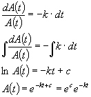
Where c is just the constant of integration. Thus, is just a constant. Let's call it A₀ and we can see that

(3)

What does A₀ physically represent? Consider what this equation looks like at time zero. When t=0, e⁰=1, so A(t) = A₀. In other words, A0 is the initial concentration of A.

Now here is an interesting question -- How did e get into all of this anyway? We have seen e pop up in thermodynamic equations before. Mathematically, of course, it came from the integral of (or in this case , but there is no mathematical need to leave eq. (3) in terms of e. We could write

(4)

Why not define things this way? 2 is a much easier number to remember than e. The reason is directly related to the definition of k given above. The first order rate constant will only have the physically meaningful identity of a true instantaneous probability if the integrated time dependence expression is phrased in terms of e. This is why in physics e always pops up in situations were the change in one parameter can be related to the value of another in terms of a probability density. Another example common in chemistry is thermal distributions such as . You can think of the equilibrium constant as the result of a thermal distribution that defines the probability of being in the initial vs. the final state. It's really the same kind of problem.

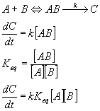
Next lets consider a simple second order reaction:

The way chemists normally think about this, it is usually broken down into two processes (more on the theory behind this idea later):

where is a collision complex between A and B. The second part is simple. That is essentially just the first order reaction we talked about above, one complex, , changes to another with some instantaneous probability, k. However, this probability must be multiplied by the probability that any particular molecule (lets consider this from the point of view of the A molecules) will be in the complex form during an interval of time, dt. What we can do now is to define some interaction volume around B and define any A molecule that is within that volume to be part of a collision complex with B. We now have a choice about how we want to think about the reaction. It could be that the reaction occurs every time that A comes within B's interaction volume or it could be that A will pass in and out of B's interaction volume many times before the reaction occurs. This will change the molecular interpretation of the rate constants but not their form. For simplicity, we will assume now that the collisions are elastic, that is, that A rapidly bounces off of B and only remains in the interaction volume for a period which is short compared to the inverse of the first order rate constant of the second part of the reaction. In this case, the overall spatial distribution of A relative to B will always be random and we can use the molar interaction volume to determine the number of A molecules which are interacting with B:

A x (Fraction of A within B's interaction volume)

Fraction of A within B's interaction volume = B x (B's molar interaction volume)

so, A x B x (B's molar interaction volume) (5)

Note that we express A and B in terms of concentrations (moles/liter) and B's molar interaction volume in liters per mole, so the units of the right side of the equation are correct (a simple concentration).

Now using the first order rate expression for formation of product:

(6)

and substituting in eq. 5:

(7)

Where VB is the molar interaction volume of B. We normally refer to as the second order rate constant for the reaction. Note that the specific interpretation of the second order rate constant as the product of a true instantaneous probability and a molar interaction volume is dependent on the assumptions that the collisions between A and B are elastic and not usually productive (many collisions are required before a reaction occurs). If we relax these assumptions, the rate equation still has the same form, but the molecular interpretation of the second order rate constant is somewhat different. Also note that the molar interaction volume of A and B are by definition the same (since this volume only applies to interactions between A and B and this interaction is symmetric). Thus, it makes no difference whether we look at the problem from the point of view of molecule A or from the point of view of molecule B.

The order of a reaction. I have been loosely talking above about first and second order reactions. I spoke of reaction order as though it could be determined by the number of chemical species that had to come together in order for the reaction to occur. In fact, reaction order is really an empirical quantity which does not even need to be an integer. It is simply given by the sum of all the exponents on the concentration terms in equations like

if one finds that in fact emprically this equation is true (regardless of what the chemical reaction equation looks like) this would be called a third order reaction (the exponents are 1 + 2). The easiest way to get used to the relationship between rate, rate constants, reaction order (molecularity) and rate equations, let's consider a few examples:

Reaction	Rate equation	Units of rate constant	Reaction order (molecularity)
Aà B		s^-1	1
A+Bà C		M^-1s^-1	2
Aà B+C		s^-1	1
Aß à B		s^-1, s^-1	1,1
A+Bß à C		M^-1s^-1	2,1
A+B+Cà D		M^-2s^-1	3

Equilibrium in terms of dynamics. One of the connections between thermodynamics and kinetics is in terms of the concept of equilibrium, Thermodynamically, equilibrium is the ratio of products and reactants that results in the lowest Gibbs free energy for the system (or the point where the chemical potentials of the products and reactants are equal). Kinetically, equilbrium is the point where the rate of the forward reaction is equal to the rate of the reverse reaction: product is going to reactant at the same rate as reactant is going to product. At this point, the net change in both reactants and products is zero. For the reaction A ß à B:

In a situation where we are considering reactions that can go either direction (and all reactions can at least to some small extent), there is a forward and backwards rate constant. These can be first or second (or higher) order rate constants, depending on the chemistry. Also, the order in the two directions can be different. Aß à B+C is first order in the forward direction but second order in the reverse direction. In the case where both forward and reverse reactions are first order, Aß à B, if we call the forward rate k_f and the reverse rate k_r we can write that

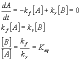
Thus, one can see that the equilibrium constant for a reaction is simply given by the ratio of the forward to reverse rate constants. As an exercise, show that this is also true for the reaction A+B ß à C (the equilibrium constant is now the ratio of the second order forward rate constant to the first order reverse rate constant). You might get a problem like this one on an upcoming exam.

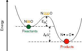
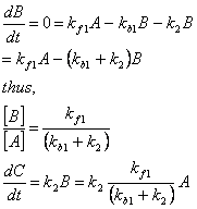
Predicting rates -- an introduction to kinetic theory. What we have discussed thus far is primarily how to take a mechanistic model and, given the rates, predict the time dependence or the concentration dependence of a chemical reaction. This is all really not based on chemistry, but rather on probability theory and the behavior of populations. The chemistry is buried in the rate constants that we use in the models. But, how does one actually predict what the molecular rate constants for a reaction would be? This is not easy to do in a quantitative sense for most chemical systems, at least not in terms of deriving an absolute value for the rate. However, we can predict with some reliability the effect of different environmental factors on the rate constants for the system. One such effect that you are probably all familiar with is the effect of temperature on rate. You have probably all seen pictures like the one given below:

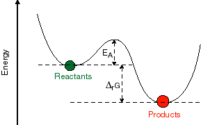What is this a picture of? It is a plot of the potential energy of the system as one progresses along the reaction coordinate connecting the initial and final state. The potential energy is the Y-axis and the reaction coordinate is the X-axis. Between the initial and final state is an energy barrier. In order to get over that barrier, energy must be put into the system from the bath. The availability of that energy is going to be very temperature dependent. This gives rise to the concept of an activation energy required to overcome the barrier and the expression:

(31)

Here EA is the activation energy and kB is the Boltzman constant. (This expression actually results from statistical mechanics. It is the probability that any individual molecule or molecular complex in the system will have an energy greater than EA which is required to overcome the barrier.) This, then, allows us to relate rates to some parameters of the energetics of the system, specifically the energetics of positions intermediate between the initial and final states of the system. But how do we think about the potential energy picture above on a molecular level and what factors will determine the activation energy for any particular reaction? One approach to understanding this is transition state theory. The basic idea is that the activation energy associated with a reaction can be attributed to the formation of a particular transition state, such as the high point between reactants (R) and Products (P) above. This could be a particular conformation of a molecule or a collision complex between molecules. Let's consider a couple of models:

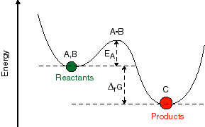In order to understand this, it is important to talk in more detail about what the reaction coordinate in these potential energy diagrams really means. The reaction coordinate that one draws in these two-dimensional pictures is some composite nuclear coordinate that is supposed to represent a change in the nuclear configuration of the chemical system which accompanies the reaction. In a very simple molecular system, such as NO, this could represent the distance between two bonded atoms. In more complex molecular systems, this coordinate may represent distance changes or orientation changes of many bonds in the system which are required to get from the reactant to the product.

In transition state theory, one talks about the progression from reactant to the product as though it occurred through a distinct intermediate in the system. This intermediate sits at the highest point in the potential surface between the reactant and product and the system can proceed in either direction from that point in the reaction. The usefulness of this concept comes from the fact that now one can suggest a particular structural model for what that transition state is and then from this predict how the rates and yields of a reaction will depend on external influences. For example, electrophillic addition to simple alkenes takes place in such a way as to form the most stable intermediate carbonium ion. Thus, more polar solvents, which will solvate and therefore stabilize this ionic intermediate, are likely to speed up such a reaction. This can be turned around from an experimentalist's point of view. If we postulate that the intermediate in a reaction is a carbonium ion, than we should see a predictable effect of solvent polarity on reaction rate. One might also be able to predict the effects of structural changes to the molecule or the presence of other molecules which might stabilize or destabilize the proposed transition state. This is a simple and elegant concept which has been the basis of many if not most of the mechanistic schemes developed for chemical reactions.

How would we predict the activation energies and rate constants of such a second order reaction? Well, that depends on exactly how the reaction worked. When we first discussed second order reactions, we talked about one way of determining the rate constant by considering the interaction volumes around A and B and estimating the probability of collision. We would then need to know how much energy was imparted by the collision. That is determined by RT.

Another approach is to look at the system as an equilibrium between the reactants and the transition state. In this case,

Here again, we can easily see the exponential dependence of rate on temperature,

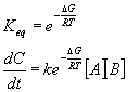
In this case, the activation energy is just the Gibbs free energy between the reactants and the transition state.

Approach to Equilibrium

Some of this I put into the notes for Chapter 10 as it seemed to fit better there (the determination of the equilibrium constant in terms of rate constants). However, there is an important extension of this that is alluded to by the book, but not described. This is the rate constant for the approach to equilibrium. Consider the simple reaction:

A ßàB

We know that dA/dt = -k_fA + k_bB (I am going to drop the concentration brackets as they get cumbersome at this point)

The question is, what does the change in concentration of A look like? We know from stochiometry that at all times A + B is a constant, call it T for total. So B = T-A. If I plug this into the equation above I can solve:

dA/dt = -k_fA + k_b(T-A) = -(k_f + k_b)A + k_bT

Note this is just a first order rate equation plus a constant (k_bT is constant since T is the total and never changes).

I can solve this differential equation (assuming that I start with all A) and get:

Looks complicated, but actually it is very easy to solve once you are used to the kinds of differential equations that appear in kinetic equations. You will not be required to solve anything this complex (you should be able to integrate the simple first order expressions). If you want to know how to solve the more complex differential equation above, come see me. But let’s look at this equation. At t=0, it has the value A₀ (which is the definition of A₀). Notice that when t=0, most of the exponential term and the constant term cancel, leaving just 1 x A₀. It then decays exponentially, just like a normal first order reaction, but the exponential decay rate constant is not k_f but rather the SUM of the forward and backward rate constants. For a reaction that is first order in both directions, this is always true. Finally at long time, the exponential term goes to zero and we are left with the constant term which is just the equilibrium value of A in terms of the total of A and B (T). Can you see why this is so?

Reaction Sequences.

Many of the more interesting reactions you will come across do not occur as a simple single reaction, but in fact occur as a series of reactions. Let's consider a reaction.

A ß à B+C ß à D

For this case lets consider the first forward reaction to have a rate constant of k_f1, the first backward reaction to have the rate constant k_b1, the second forward rate constant is k_f2 and the second backward rate constant is k_b2. How do we describe the kinetics of this reaction? We can always write down the rate equations for each species in the reaction, assuming that these are elementary reactions which are an accurate representation of the reaction mechanism (this is something you should be prepared to do):

By the way, you should also be able to tell me the initial rate of change in the concentrations of A, B, C and D if you are given the initial concentrations of each and the values of the rate constants.

But how do we go farther than this to determine the actual concentration time dependence? The answer is that we can either solve these differential equations directly (which can be done for this case, but is messy) or we can make some simplifying assumptions and reduce it down to a simpler case.

For rate equations up to about the complication of the one in the example above, it is fairly straightforward to solve the equations exactly, especially if one uses programs such as Maple or MathCad to help with the algebra. More complex series of chemical reactions often have no analytical solution. In these cases we have two choices. We can either solve our problem numerically (calculate the change in concentration for a small change in time, update the concentrations and recalculate for the next time increment, etc.) or we can use an assumption about the way that the chemical mechanism works. Here, I would like to go over three such assumptions.

Limiting rate assumption. This is probably the simplest of assumptions. Let's say I have a series of reactions that are essentially irreversible, Aà B à C. In other words, the equilibrium constants are much greater than 1. Let's also suppose that the first reaction is much faster than the second. What will be the time dependence of product formation? It will be determined simply by the slowest reaction. In this case, the time for the B to C reaction will be limiting. Thus, the overall rate of the reaction will be determined simply by the rate constant of the B to C reaction. Note that the rate of A disappearance will be determined by the rate constant of the A to B reaction. This is because it does not matter to A what happens later in the chain of reactions.

Equilibrium assumption. Here, we assume that one of the reactions comes to equilibrium very rapidly compared to the other rates in the reaction. Consider the reaction A ß à B à C. As we saw above, the rate constant for approach to equilibrium in a simple case like this is just the sum of the forward and backward rate constants of a reaction. Thus we can say in this case that if the sum of the forward and backwards rate constants for the first reaction is much faster than the rate constant for the second reaction then the first reaction will come to equilibration before much product is formed. (Generally, what follows is true any time the first reaction comes to equilibrium rapidly compared with the time scale of product formation.)

here k₂ is the rate constant for the second reaction and K_eq is the equilibrium constant for the first reaction. We have now reduced this series reaction to something that is mathematically like a first order reaction of A going to C, except that the effective first order rate constant is comprised of both k₂ and K_eq. Let's do a real example here. Let's say that I add one mole of A to a liter of water. I want to know what the time course of C formation is. Ok, the equilibrium assumption says that instantly A and B will come to equilibrium. Thus, the amount of A and B present just after adding A in the solution is given by the equilibrium constant. Let's suppose that the equilibrium constant is 0.01 and that the rate constant for the second reaction is 1 1/s. Thus the equilibrium concentration of A is 0.99M and that of B is 0.01M (A and B come to equilibrium instantly giving a 0.01 ratio of B to A). This means that effectively, the initial amount of A is 0.99M and the effective first order rate constant for formation of C from A is k₂K_eq = 0.01 1/s. Thus the time course is given by C(t) = 0.99M e^-(0.01)t. Note that since this reduces to a first order rate equation the integral is the same as it was for a first order rate equation previously. Note also, that this would not have been so simple if the equilibrium constant had been closer to 1. Here we were able to largely ignore the contribution of B is the overall concentration. If the equilibrium constant were closer to one, this would not have been possible.

Steady-state approximation. The steady state approximation assumes that the intermediate is present not in equilibrium with one of the other chemical species but rather in steady-state. This means that it is being used up as fast as it is formed and therefore its concentration does not change very quickly. In this case, we have that

Again, we have reduced the series of reactions to something that looks rather like a first order reaction of A forming C. Again, as long as the intermediate concentration of B is low, we can simply analyze the system as though it was a first order reaction between A and C with a first order rate constant of .

Note something important here. This expression reduces to the same thing we got in the equilibrium approximation for the special case that k_b1 >>k₂. In other words, if the equilibration rate constants are fast enough, it will come to equilibrium before there is any further reaction and the equilibrium assumption will hold. If the equilbrium rate constants are not fast enough compared to k₂ then we must use the steady state assumption.

Problems done in class on photosynthesis and transcription