
Project: Dynamic Heterogeneity |
|
Dynamical heterogeneity refers to the observation of spatially varying time scales of molecular rearrangements (or viscosities) in single component liquids [106, 190]. For example, the time molecules require for reorientation can differ by a factor of 100 for two positions which are only a few nanometers apart. Dynamic heterogeneity is the source of several new questions: What is the length scale and persistence time associated with such clusters of relaxation time? What is the signature of heterogeneity at high temperatures and in the glassy state? How do these features depend on the particular material and on the correlation function used for probing these heterogeneities? |

|
Schematic representation of two different sources of non-exponential correlation decays.
The left part outlines a homogeneous relaxation scenario, in which all local
contributions are identical to the ensemble average. The right side refers
to heterogeneous dynamics, characterized by individual relaxing units having
site specific relaxation times. By virtue of the ensemble average the two
distinct relaxation models can lead to the same decay pattern if the macroscopic
response is considered. [36, 37, 106] |
|
Our experimental approach to heterogeneous dynamics is by triplet state solvation dynamics [70, 93, 102, 143], by dielectric hole burning [91, 98, 103, 112, 115], and by non-linear dielectric studies [147, 151, 157, 162, 168, 174, 185, 215]. In the solvation experiment, it is the time-resolved width of the emission spectra which is incompatible with homogeneous dynamics. Various models of solvation in viscous solvents allow us to analyse heterogeneity more quantitatively for relaxation times between 1 ms and 30 s [100, 101]. |
|
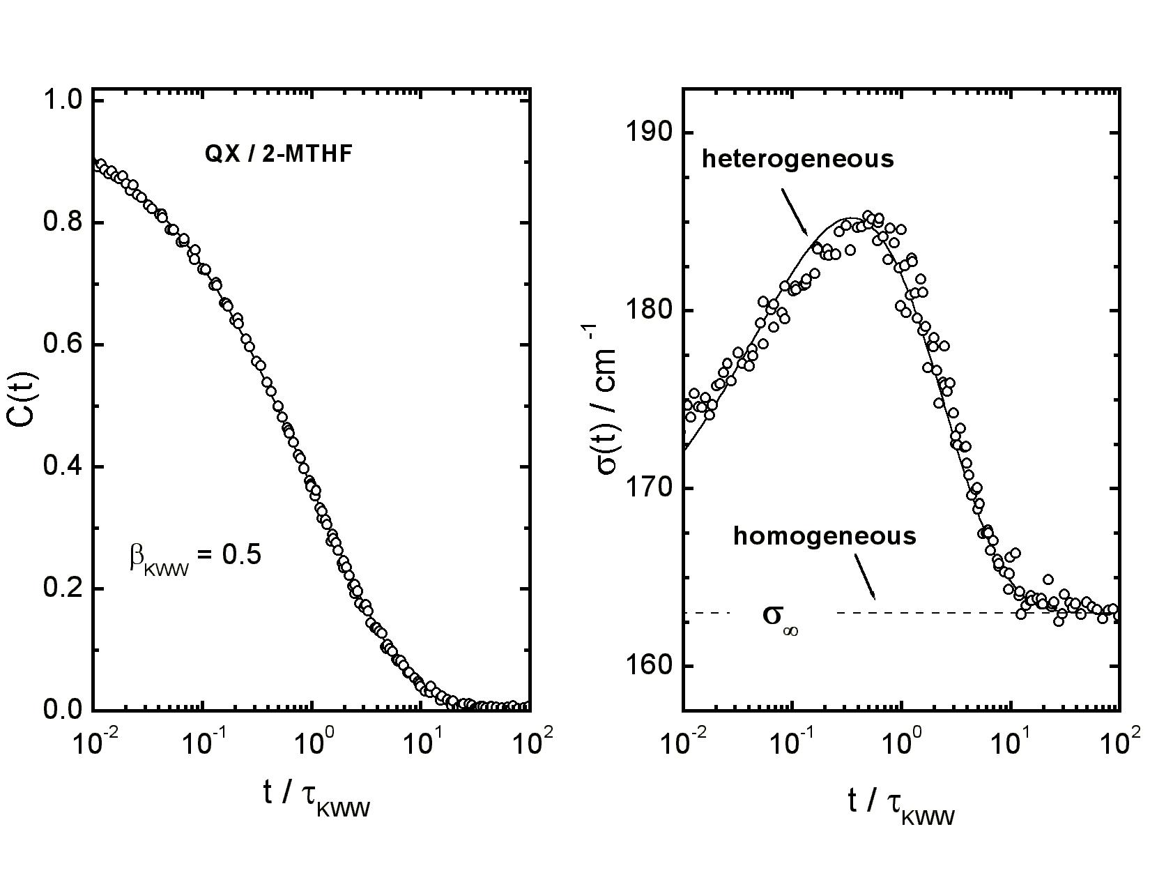
Master plot of the Stokes shift correlation function C(t) (symbols, l.h.s.) and
of the inhomogeneous linewidth σ(t) (symbols, r.h.s.) versus
t/τKWW for the solute quinoxaline in the solvent MTHF,
measured at temperatures 91 K ≤ T ≤ 97 K in steps of 1 K.
The solid line in the l.h.s. panel is a fit to C(t) using a stretched exponential
function. The solid line in the r.h.s. panel is based upon dynamic heterogeneity,
whereas homogeneity would lead to σ(t) = σ∞. [81, 93, 96, 143]
|
|
A similar method employing shorter lived fluorescence probes has revealed dynamic heterogeneity also at higher temperatures, where the relaxation time is a few nanoseconds [102]. |

|
It has been observed by time-resolved non-linear dielectric spectroscopy that the
equilibration of time-constants (the process of rate exchange) occurs on the time
scale of the average α-relaxation time, even for modes in the excess wing that
are 107 times faster than the most probable time constant. [215] Schematic representation of heterogeneity in terms of five distinct Debye type modes whose superposition yields a dispersive dielectric loss peak. Arrows in the top part indicate the equilibration of fictive temperatures or relaxation time constants, the process of an aging isotherm occurring in response to a temperature down-jump. Arrows in the bottom part indicate rate exchange at a constant temperature. The two scenarios are linked only qualitatively by the fluctuation dissipation theorem (FDT). [215] |
|
Reference numbers refer to the list of publications |
|
Experimental techniques:
|
Selected projects:
|