Simulation of hillslope processes using Microsoft Excel

Due:  at the beginning of class, November 22, 2000.

Modified November 10, 2000.

Purpose: These laboratory exercises are designed to help you gain appreciation for modeling of hillslope processes.
I have prepared this excel file for you:
simplediffusion.xls Original from Thursday Lab demo.
simplediffusion2.xls Cleaned up spreadsheet. It is comprised of two sheets: Interface--on which you should do your work; and Model Calculations--second sheet with all of the model calculations so as to cut down on clutter.

Queen Creek

The variables you have to watch are these:

These are ones you change:
dx    The horizontal distance between the elevation measurements that make up a profile.  
      This can be changed to alter the length of the profile but it is constant for every portion of any profile.
dt    The time between each calculation step.  There are 573 calculation steps in this model.  
      You change this number to define the total age of the profile (dt*573).
k     This is the transport rate for our assumed transport law.  We discussed independent measurements of this 
      parameter that seem to vary generally with current climate such that very dry places like Israel have 
      k = 0.1  m^2/ka; the US Basin and Range have k = 1 m^2/ka; and California and Michigan have k = 10 m^2/ka.
Individual change per timestep.  Whatever goes into this cell will be added to the elevation for that 
      position each time step.
Initial elevations    Elevations at the beginning of the time of interest that is modelled.
Hobserved     Observed final elevations

Here ones that are calculated:
Hmodel (Final model elevations) Elevations that change as a result of the modeling.
RMS =  root mean square error  
       The equation for this is rms = SQRT(1/p(sum(Hobserved - Hmodel)[summed for all cells in  the entire profile])^2))
       
       Where where p is the number of observations, Hi is the observed value at xi, and Hmodel(xi) 
       is the model or calculated value at xi.
       It has units of elevation (meters) in this case.  It is a measure of the average distance between the modeled 
       elevations and the observed ones.  The best fitting profile is defined as the one which causes the minimum RMS

lambda = (k*dt(dx^2).  
       This is a measure of stability for the numerical model and is only for diagnosis purposes.  
       It must be <0.5 for this modeling to work.

1)  Using the idealized ramp initial form, make a plot showing the initial form and final forms for t = 1 ka, and k = 1 m2/ka;  t = 5 ka, and k = 1 m2/ka;  t = 10 ka, and k = 1 m2/ka;  t = 1 ka, and k = 10 m2/ka.  Discuss the effects of varying t and k on the final form. HINT:  look at the product k•t.

3)  Try different initial conditions. What are some other forms that might be interesting to see what happens as they change shape?

4)  What happens if one of the boundaries drops at a constant rate?  Change the Individual change per timestep column for just the lower or upper end. Is the initial form important in the development of the final form?

5)  What happens with a constantly offsetting surface (fault) in the center of the profile?  Use the Individual change per timestep and change the lower half of the profile to a small negative number (offset per time step). Be sure to try different offset rates.  Note that this could give a problem with slopes > the angle of repose, but should not be too great of a problem.

6)  Try deposition over the lower portion of the profile (similar to above implementation (but with a positive number for the Individual change per timestep
 for a given cell).  What effect on the final form is there from deposition?  Be sure to try different deposition rates.

7)  Using the Queen creek data we gathered for the upper and lower risers, estimate the age of the upper riser (age of the middle surface).  Do this by generalizing the observations of the lower riser as the original profile.  Use its steepness and curvature but apply that to the height of the upper riser.  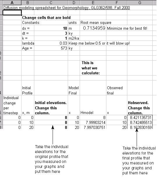Divide the profile into equally spaced segments (27) and figure out what the dx will be and then determine an original and final observed elevation for each node (cell) and input that into the excel spreadsheet below.  Make an assumption about the diffusivity (k) and then adjust the dt (which controls the final age) to minimize the RMS error and thus determine the best age for the riser.
Here is the spreadsheet for this problem:
 simplediffusionwithdata.xls
-->simplediffusionwithdata2.xls Cleaned up spreadsheet. It is comprised of two sheets: Interface--on which you should do your work; and Model Calculations--second sheet with all of the model calculations so as to cut down on clutter.

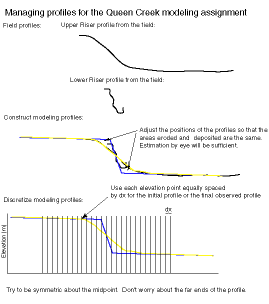
Below is a graphic about how to prepare the profiles for modeling. It will will help you to make some decisions about how to get the elevations you need to put into the spreadsheet.

You have to choose a dx that balances the distance covered (dx*28; note there are 28 actual nodes) with the detail on the scarp. As I point out above, you just need to cover the portion of the scarp where things are happening. Perhaps go a bit further out so as to allow the model calculations to not get hung up on the constant elevation boundaries.

Here is then where to put those elevations:


Questions:

How old is the riser?  What is your estimate of uncertainty on that number?  How good is the age in other words?  What is the plus-minus on that age?
What k did you use and what is the justification for it?
What assumptions are essential for this analysis and how good are they for this case?
 
Incomplete list of references to publications that used this method to do something important